Voltage collapse prediction for interconnected power systems

Graduate Theses, Dissertations, and Problem Reports

2000

Voltage collapse prediction for interconnected power systems Voltage collapse prediction for interconnected power systems

Amer S. Al-Hinai

West Virginia University

Follow this and additional works at: https://researchrepository.wvu.edu/etd

Recommended Citation Recommended Citation

Al-Hinai, Amer S., "Voltage collapse prediction for interconnected power systems" (2000).

Graduate

Theses, Dissertations, and Problem Reports

. 1065.

https://researchrepository.wvu.edu/etd/1065

This Thesis is protected by copyright and/or related rights. It has been brought to you by the The Research

Repository @ WVU with permission from the rights-holder(s). You are free to use this Thesis in any way that is

permitted by the copyright and related rights legislation that applies to your use. For other uses you must obtain

permission from the rights-holder(s) directly, unless additional rights are indicated by a Creative Commons license

in the record and/ or on the work itself. This Thesis has been accepted for inclusion in WVU Graduate Theses,

Dissertations, and Problem Reports collection by an authorized administrator of The Research Repository @ WVU.

For more information, please contact researchreposit[email protected].

VOLTAGE COLLAPSE PREDICTION FOR INTERCONNECTED POWER

SYSTEMS

Amer AL-Hinai

Thesis submitted to College of Engineering

and Mineral Resources at West Virginia University

in partial fulfillment of the requirements for

the degree of

Master of Science

In

Electrical Engineering

Muhammad A. Choudhry, Ph.D., Chair

Ali Feliachi, Ph.D.

Ronald L. Klein, Ph. D.

Morgantown, West Virginia

2000

Keywords: Power Systems, Voltage Collapse, Modal Analysis, Q-V Curve, Load Characteristics

and Induction Machine Load.

ABSTRACT

VOLTAGE COLLAPSE PREDICTION FOR INTERCONNECTED POWER SYSTEMS

Amer AL-Hinai

A steady state analysis is applied to study the voltage collapse problem. The modal analysis

method is used to investigate the stability of the power system. Q-V curves are used to confirm the

obtained results by modal analysis method and to predict the stability margin or distance to voltage

collapse based on reactive power load demand. The load characteristics are considered in this

research. Different voltage dependent loads are proposed in order to be used instead of the

constant load model. The effect of induction machine load is considered in this study. The load is

connected to several selected buses.

The analysis is performed for three well-known system; Western System Coordinating Council

(WSCC) 3-Machines 9-Bus system, IEEE 14 Bus system and IEEE 30 Bus system. The modal

analysis technique is performed for all systems using the constant load model, the voltage

dependent load models and induction machine load model. Then, the most critical mode is

identified for each system. After that, the weakest buses, which contribute the most to the critical

mode, are identified using the participation factor. The Q-V curves are generated at specific buses

in order to check the results obtained by the modal analysis technique and to estimate the stability

margin or distance to voltage collapse at those buses.

iii

ACKNOWLEDGEMENTS

First I would like to express my sincere appreciation to my research advisor Prof. Muhammad

Choudhary for his support and guidance of this research. I would like also to thank Prof. Ali

Feliachi for his advice and direction. My thanks are extended to Prof. Ronald Kline for his

suggestion and advice. My special thanks are expressed to Dr. Khaled Elithiy (Sultan Qaboos

University) for helpful advice, encouragements and discussions.

Thanks are also to Sultan Qaboos University for giving me full financial support throughout my

education.

Special thanks to my wife for her support, help and patience while we are away from our home

country, Oman. Finally, I would like to thank my mother, my brothers, and my sister for their help

and encouragements.

iv

DEDICATION

To my mother,

To my brothers and my sister,

To my wife.

v

TABLE OF CONTENTS

ABSTRACT.................................................................................................................ii

ACKNOWLEDGEMENTS........................................................................................iii

DEDICATION............................................................................................................iv

TABLE OF CONTENTS ............................................................................................ v

LIST OF FIGURES..................................................................................................viii

LIST OF TABLES......................................................................................................xi

CHAPTER 1

INTRODUCTION

1.1 Introduction and Background................................................................................ 1

1.2 Scope of Thesis...................................................................................................... 3

CHAPTER 2

LITERATURE REVIEW

2.1 Introduction............................................................................................................ 5

2.2 Dynamic and Steady State Analysis...................................................................... 7

2.3 Methods of Voltage Stability Analysis.................................................................. 9

2.3.1 Q-V Curve ......................................................................................................... 9

2.3.2 P-V curve......................................................................................................... 10

2.3.3 Multiple Power Flow Solutions....................................................................... 11

2.3.4 Minimum Singular Value Decomposition. ..................................................... 12

2.3.5 Modal or Eigenvalue Analysis Method........................................................... 12

2.4 Power Flow Problem ........................................................................................... 13

CHAPTER 3

METHOD OF ANALYSIS

3.1 Introduction.......................................................................................................... 16

3.2 Modal Analysis.................................................................................................... 16

3.3 Identification of the Weak Load Buses ............................................................... 20

vi

3.4 Q-V Curve ........................................................................................................... 22

3.5 Effect of Load Modeling ..................................................................................... 24

3.5.1 Voltage Dependent Load................................................................................. 25

3.6 Effect of Induction Motor Load. ......................................................................... 26

CHAPTER 4

RESULTS AND DISCUSSION

4.1 Introduction......................................................................................................... 28

4.2 Test Systems Description .................................................................................... 28

4.3 Analysis with Constant Impedance Load............................................................ 30

4.3.1 Western System Coordinating Council (WSCC) 3-Machines 9-Bus system. 30

4.3.2 The IEEE 14 Bus system................................................................................. 34

4.3.3 The IEEE 30 Bus system................................................................................. 36

4.4 Analysis Considering Load Characteristics. ....................................................... 40

4.4.1 Western System Coordinating Council (WSCC) 3-Machines 9-Bus system. 40

4.4.2 The IEEE 14 Bus system................................................................................. 45

4.4.3 The IEEE 30 Bus system................................................................................. 48

4.5 Analysis Considering Effect of Induction Machine Load................................... 52

4.5.1 Western System Coordinating Council (WSCC) 3-Machines 9-Bus system. 53

4.5.2 The IEEE 14 Bus system................................................................................. 56

4.5.3 The IEEE 30 Bus system................................................................................. 60

CHAPTER 5

CONCLUSION & RECOMMENDATIONS

5.1 Conclusion........................................................................................................... 64

5.2 Recommendations for the Future Research......................................................... 65

REFERENCES

References……………………………………………………………………...…...67

vii

APPENDIX A

A.1 Test Systems Load Flow Data........................................................................... 68

A.1.1 WSCC system Load Flow Data...................................................................... 68

A.1.2 IEEE 14 Bus System Load Flow Data............................................................ 69

A.1.3 IEEE 30 Bus System Load Flow Data............................................................ 70

A.2 Load Flow Solution. .......................................................................................... 72

A.2.1 WSCC system Load Flow Solution with Constant Load Model.................... 72

A.2.2 IEEE 14 Bus System Load Flow Solution with Constant Load Model. ........ 73

A.2.3 IEEE 30 Bus System Load Flow Solution with Constant Load Model. ........ 74

APPENDIX B

B.1 Analysis Program................................................................................................ 77

B.2 Load Flow Program ............................................................................................ 85

viii

LIST OF FIGURES

Figure 2.1 Typical P-V curve...........................................................................................................11

Figure 3.1 Algorithm for the voltage stability analysis....................................................................21

Figure 3.2 Typical Q-V curve..........................................................................................................24

Figure 4.1 Western System Coordinating Council (WSCC) 3-Machines 9-Bus system.................29

Figure 4.2 Single line diagram of the IEEE 14 Bus System............................................................29

Figure 4.3 Single line diagram of the IEEE 30 Bus System............................................................30

Figure 4.4 Voltage profiles of all buses of the WSCC 3-Machines 9-Bus system..........................31

Figure 4.5 The participating factor of all buses for most critical mode for the WSCC 3-Machines

9-Bus system............................................................................................................................32

Figure 4.6 The Q-V curves at buses 5, 8 and 6 for the WSCC 3-Machines 9-Bus system. ............33

Figure 4.7 Voltage profiles of all buses of the IEEE 14 Bus system...............................................34

Figure 4.8 The participating factor of all buses for most critical mode for the IEEE 14 Bus system.

..................................................................................................................................................35

Figure 4.9 The Q-V curves at buses 9, 10 and 14 for the IEEE 14 Bus system. .............................36

Figure 4.10 Voltage profiles of all buses of the IEEE 30 Bus system.............................................37

Figure 4.11 The participating factor of all buses for most critical mode for the IEEE 30 Bus

system.......................................................................................................................................39

Figure 4.12 The Q-V curves at buses 30, 29 and 26 for the IEEE 30 Bus system. .........................39

Figure 4.13 Voltage profiles of all buses of the WSCC 3-Machines 9-Bus system at different load

models......................................................................................................................................41

Figure 4.14 The participating factor of all buses for most critical modes for the WSCC 3-Machines

9-Bus system at different load models.....................................................................................41

Figure 4.15 The Q-V curves at bus 5 for the WSCC 3-Machines 9-Bus system at different load

models......................................................................................................................................42

Figure 4.16 The Q-V curves at bus 6 for the WSCC 3-Machines 9-Bus system at different load

models......................................................................................................................................43

Figure 4.17 The Q-V curves at bus 5 for the WSCC 3-Machines 9-Bus system at different load

models (Unstable system). .......................................................................................................44

Figure 4.18 The Q-V curves at bus 6 for the WSCC 3-Machines 9-Bus system at different load

models (Unstable system). .......................................................................................................44

ix

Figure 4.19 Voltage profiles of all buses of the IEEE 14 Bus system at different load’s models...46

Figure 4.20 The participating factor of all buses for most critical modes for the IEEE 14 Bus

system at different load’s models.............................................................................................47

Figure 4.21 The Q-V curves at bus 14 for the IEEE 14 Bus system at different load’s models......47

Figure 4.22 The Q-V curves at bus 14 for the IEEE 14 Bus system at different load models

(Unstable system).....................................................................................................................48

Figure 4.23 Voltage profiles of all buses of the IEEE 30 Bus system at different types of load

models......................................................................................................................................50

Figure 4.24 The participating factor of all buses for most critical modes for the IEEE 30 Bus at

different types of load models..................................................................................................50

Figure 4.25 The Q-V curves at bus 30 for the IEEE 30 Bus system at different types of load.......51

Figure 4.26 The Q-V curves at bus 30 for the IEEE 30 Bus system at different load’s models

(Unstable system).....................................................................................................................52

Figure 4.27 Voltage profiles of all buses of the WSCC 3-Machines 9-Bus system including

Induction machine load at bus # 5. ..........................................................................................53

Figure 4.28 The participating factor of all buses for the most critical modes for the WSCC 3-

Machines 9-Bus system at different load models at bus # 5....................................................54

Figure 4.29 The Q-V curves at bus 5 for the WSCC 3-Machines 9-Bus system at different load

models at bus# 5.......................................................................................................................55

Figure 4.30 The Q-V curves of bus # 5 for the WSCC 3-Machines 9-Bus system at different

induction machine load models (Unstable system)..................................................................56

Figure 4.31 Voltage profiles of all buses of the IEEE 14 Bus system including Induction machine

load at bus # 14. .......................................................................................................................57

Figure 4.32 The participating factor of all buses for most critical modes for the IEEE 14 Bus

System at different load’s models in bus # 14. ........................................................................58

Figure 4.33 The Q-V curves at bus # 14 for the IEEE 14 Bus System at different load’s models in

bus # 14....................................................................................................................................59

Figure 4.34 The Q-V curves of bus # 14 for the IEEE 14 Bus system at different induction

machine load’s models at bus # 14 (Unstable system). ...........................................................59

Figure 4.35 Voltage profiles of all buses of the IEEE 30 Bus system including Induction machine

load at bus # 30. .......................................................................................................................60

x

Figure 4.36 The participating factor of all buses for most critical modes for the IEEE 30 Bus

System at different load models at bus # 30. ...........................................................................62

Figure 4.37 The Q-V curves at bus # 30 for the IEEE 30 Bus System at different load’s models in

bus # 30....................................................................................................................................62

Figure 4.38 The Q-V curves of bus # 30 for the IEEE 30 Bus system at different induction

machine load models at bus # 30 (Unstable system)...............................................................63

xi

LIST OF TABLES

Table 2.1 Voltage collapse incidents. ................................................................................................6

Table 2.2 Incidents without collapse..................................................................................................7

Table 4.1 WSCC 3-Machines 9-Bus system eigenvalues................................................................31

Table 4.2 Voltage and reactive power margins for the WSCC 3-Machines 9-Bus system from Q-V

curves. ......................................................................................................................................33

Table 4.3 IEEE 14 Bus system eigenvalues.....................................................................................34

Table 4.4 Voltage and reactive power margins for the IEEE 14 Bus system from Q-V curves......36

Table 4.5 IEEE 30 Bus system eigenvalues sorted by ascending values.........................................38

Table 4.6 Voltage and reactive power margins for the IEEE 30 Bus system from Q-V curves......38

Table 4.7 WSCC 3-Machines 9-Bus system eigenvalues at different np and nq values. ................40

Table 4.8 Voltage and reactive power margins for the WSCC system from Q-V curves for bus # 5.

..................................................................................................................................................43

Table 4.9 Voltage and reactive power margins for the WSCC system from Q-V curves for bus # 6.

..................................................................................................................................................43

Table 4.10 IEEE 14 Bus system eigenvalues at different np and nq values....................................45

Table 4.11 Voltage and reactive power margins for the IEEE 14 Bus system from Q-V curves for

bus # 14....................................................................................................................................48

Table 4.12 IEEE 30 Bus system eigenvalues at different np and nq values....................................49

Table 4.13 Voltage and reactive power margins for the IEEE 30 Bus system from Q-V curves for

bus # 30....................................................................................................................................51

Table 3.14 Induction machine parameters. ......................................................................................53

Table 4.15 WSCC 3-Machines 9-Bus system eigenvalues at different loads in bus # 5.................54

Table 4.16 Voltage and reactive power margins for the WSCC system from Q-V curves for bus# 5.

..................................................................................................................................................55

Table 4.17 IEEE 14 Bus system eigenvalues at different loads at bus # 14....................................57

Table 4.18 Voltage and reactive power margins for the IEEE 14 Bus system from Q-V curves for

bus # 14....................................................................................................................................58

Table 4.19 IEEE 30 Bus system eigenvalues at different loads at bus # 30....................................61

xii

Table 4.20 Voltage and reactive power margins for the IEEE 30 Bus system from Q-V curves for

bus # 30....................................................................................................................................63

CHAPTER 1 INTRODUCTION

1

CHAPTER 1

INTRODUCTION

1.1 Introduction and Background

Voltage collapse problem has been one of the major problems facing the electric power utilities in

many countries. The problem is also a main concern in power system operation and planning. It

can be characterized by a continuous decrease of the system voltage. In the initial stage the

decrease of the system voltage starts gradually and then decreases rapidly. The following can be

considered the main contributing factors to the problem [22]:

1. Stressed power system; i.e. high active power loading in the system.

2. Inadequate reactive power resources.

3. Load characteristics at low voltage magnitudes and their difference from those traditionally

used in stability studies.

4. Transformers tap changer responding to decreasing voltage magnitudes at the load buses.

5. Unexpected and or unwanted relay operation may occur during conditions with decreased

voltage magnitudes.

This problem is a dynamic phenomenon and transient stability simulation may be used. However,

such simulations do not readily provide sensitivity information or the degree of stability. They are

also time consuming in terms of computers and engineering effort required for analysis of results.

The problem regularly requires inspection of a wide range of system conditions and a large

number of contingencies. For such application, the steady state analysis approach is much more

suitable and can provide much insight into the voltage and reactive power loads problem [20] and

[13].

CHAPTER 1 INTRODUCTION

2

So, there is a requirement to have an analytical method, which can predict the voltage collapse

problem in a power system. As a result, considerable attention has been given to this problem by

many power system researchers. A number of techniques have been proposed in the literature for

the analysis of this problem [5].

The problem of reactive power and voltage control is well known and is considered by many

researchers. It is known that to maintain an acceptable system voltage profile, a sufficient reactive

support at appropriate locations must be found. Nevertheless, maintaining a good voltage profile

does not automatically guarantee voltage stability. On the other hand, low voltage although

frequently associated with voltage instability is not necessarily its cause [15] and [32].

In 1992 Geo, Morison and Kundur proposed the Modal analysis technique to predict the voltage

collapse of a power system. The method basically computes the smallest eigenvalue and associated

eigenvectors of the reduced Jacobian matrix of the power system based on the steady state system

model. The eigenvalues are associated with a mode of voltage and reactive power variation. The

system stability can be evaluated by checking the status of those eigenvalues. If all the eigenvalues

are positive, then the system is considered to be voltage stable. On the other hand, the system is

considered to be voltage unstable if only one of the eigenvalues is negative. A zero eigenvalue of

the reduced Jacobian matrix means that the system is on the border of voltage instability. The

potential voltage collapse situation of a stable system can be predicted through the evaluation of

the minimum positive eigenvalues. The magnitude of each minimum eigenvalue provides a

measure how close the system is to voltage collapse.

By using the participation factor, the weakest bus or node can be determined which is the greatest

contributing factor for a system to reach voltage collapse situation. This can provide insight into

possible remedial action as well as contingencies, which may result in losing the system.

CHAPTER 1 INTRODUCTION

3

Q-V curve is a general method used by many utilities to assess the voltage stability. It can be used

to determine proximity to voltage collapse since it directly assesses shortage of reactive power.

The curves mainly show the sensitivity and variation of bus voltage with respect to reactive power

injection. Using the Q-V curves, the stability margin or distance to voltage collapse at a specific

bus can be evaluated.

It is common in steady state analysis to represent the loads by a combination of constant

impedance, constant current and constant power elements. However, it is found that voltage

stability analysis is affected by considering the load characteristics. The importance of proper

representation of loads in power system stability studies has been noticed clearly.

The induction machine is one of the most important loads in a power system especially in the

industrial area. It has been found that, such load can influence the system voltage stability in a

wide range. As a result, considerable attention has been taken by many power system researchers

regarding this load.

1.2 Scope of Thesis.

In chapter 2, a literature review is presented, discussing the voltage collapse problem in an electric

power system. Many voltage instability incidents have occurred around the world. Lists of

incidents resulting in voltage collapse and not resulting in voltage collapse are presented. Then, a

number of related published techniques have been discussed briefly.

In chapter 3, the modal or eigenvalue analysis technique is discussed. The method is used to

provide a relative measure of proximity to voltage instability. The load characteristics are also

discussed in this chapter. A voltage dependent load model is proposed to be used for the analysis.

In addition, the induction machine load model effect is considered. The model is derived from the

steady state equivalent circuit of induction machine. The active and reactive powers consumed by

the induction motor are function of the bus voltage and machine slip.

CHAPTER 1 INTRODUCTION

4

In chapter 4, the research results are presented. First, the analysis is applied using the constant load

model. Then, different voltage dependent load models are applied and the results analyzed. After

that, the induction machine load model is connected to selected buses in the systems. The

preceding analyses is applied with the new load model.

In chapter 5, the research conclusion is presented and the recommendations are made for further

work.

CHAPTER 2 LITERATURE REVIEW

5

CHAPTER 2

LITERATURE REVIEW

2.1 Introduction

Recently, increased attention has been devoted to the voltage instability phenomenon in power

systems. Voltage stability is concerned with the ability of a power system to maintain acceptable

voltage level at all nodes in the system under normal and contingent conditions. A power system is

said to have a situation of voltage instability when a disturbance causes a progressive and

uncontrollable decrease in voltage level. The voltage instability progress is usually caused by a

disturbance or change in operating conditions, which create increased demand for reactive power

[9] and [30]. This increase in electric power demand makes the power system work close to their

limit conditions such as high line current, low voltage level and relatively high power angle

differences which indicate the system is operating under heavy loading conditions. Such a

situation may cause losing system stability, islanding or voltage collapse.

The main problem facing many utilities in maintaining adequate voltage level is economic. They

are squeezing the maximum possible capacity for their bulk transmission network to avoid the cost

of building new lines and generation facilities. When a bulk transmission network is operated close

to the voltage instability limit, it becomes difficult to control the reactive power margin for that

system. As a result the system stability becomes one of the major concerns and an appropriate way

must be found to monitor the system and avoid system collapse [33].

One of the major reasons of voltage collapse is the heavy loading of the power system, which is

comprised of long transmission lines. The system appears unable to supply the reactive power

demand. Producing the demanded reactive power through synchronous generators, synchronous

condensers or static capacitors, can overtake the problem [7]. Another solution is to build

CHAPTER 2 LITERATURE REVIEW

6

Table 2.1 Voltage collapse incidents.

Date Location Duration

13April1986

Winnipeg, Canada

Nelson River HVDC link

1 second

30Nov.1986 SE Brazil, Paraguay 2 seconds

17May1985 South Florida 4 seconds

22Aug.1987 Western Tennessee 10 seconds

27Dec.1983 Sweden 55 seconds

21May1983 Northern California 2 minutes

2Sep.1982 Florida 1-3 minutes

26Nov.1982 Florida 1-3 minutes

28Dec.1982 Florida 1-3 minutes

30Dec.1982 Florida 1-3 minutes

22Sep.1977 Jacksonville, Florida Few minutes

4Aug.1982 Belgium 4.5 minutes

20May1986 England 5 minutes

12Jan.1987 Western France 6-7 minutes

9Dec.1965 Brittany, France Unknown

10Nov.1976 Brittany, France Unknown

23July1987 Tokyo 20 minutes

19Dec.1978 France 26 minutes

22Aug.1970 Japan 30 minutes

22Sep.1970 New York State Several hours

20July1987 Illinois and Indiana Hours

11June1984 Northeast United States Hours

transmission lines to the weakest nodes. Voltage collapse may occur due to a major disturbance in

the system such as generators outage or lines outage. In such a situation a protection system and

proper control may resolve the problem.

CHAPTER 2 LITERATURE REVIEW

7

Many voltage collapse incidents have occurred throughout the world as shown in Table 2.1 and

Table 2.2 [1].

Table 2.2 Incidents without collapse.

Date Location Duration

17,20,21May1986

Miles City, Montana, USA

HVDC link

Transient, 1-2 second

11,30,31July1987 Mississippi, USA Transient, 1-2 seconds

11July1989 South Carolina, USA Unknown

21May1983 North California, USA Longer term, 2 minutes

10Aug.1981 Longview, Wash., USA Longer term, minutes

17Sept.1981 Central Oregon, USA Longer term, minutes

20May1986 England Longer term, 5minutes

2Mar.1979 Zealand, Denmark Longer term, 15minutes

3Feb.1990 Western France Longer term, minutes

Nov.1990 Western France Longer term, minutes

22Sept.1970 New York state, USA

Longer term, minutes insecure

for hours

20July1987 Illinois and Indiana, USA

Longer term, minutes insecure

for hours

11June1984 Northeast USA

Longer term, minutes insecure

for hours

5July1990 Baltimore, Washington D.C,

USA

Longer term, minutes insecure

for hours

2.2 Dynamic and Steady State Analysis

Voltage stability analysis involves both steady state and dynamic aspects [21]. Researchers have

used both approaches. The Steady State or Static Methods mainly depend on the steady state

model in the analysis, such as power flow model or a linearized dynamic model described by the

steady state operation. These methods can be divided into [1], [34] and [12]:

1. Load flow feasibility methods, which depend on the existence of an acceptable voltage

profile across the network. This approach is concerned with the maximum power transfer

CHAPTER 2 LITERATURE REVIEW

8

capability of the network or the existence of a solved load flow case. There are many

criteria proposed under this approach. Some of these criteria are the following:

- The reactive power capability (Q-V curve).

- Maximum power transfer limit (P-V curve).

- Voltage instability proximity index or the load flow feasibility index (LFF index).

2. Steady state stability methods, which test the existence of a stable equilibrium operating

point of the power system. Some of the criteria proposed under this approach are:

- Eigenvalues of linearized dynamic equations (ELD).

- Singular value of Jacobian matrix (SVJ).

- Sensitivity matrices.

It is well known that voltage stability is indeed a dynamic phenomenon. The dynamic analysis

implies the use of a model characterized by nonlinear differential and algebraic equations which

include generators dynamics, induction motor loads, tap changing transformers, etc... through

transient stability simulations. However, such simulations do not readily provide sensitivity

information or the degree of stability. They are also time consuming in terms of computers speed

and engineering required for analysis of results. Therefore, the dynamic simulation applications

are limited to investigation of specific voltage collapse situations, which include fast or transient

voltage collapse. Also, it is used for coordination of protection systems and controls.

On the other hand, voltage stability analysis regularly requires inspection of a wide range of the

system conditions and a large number of contingency circumstances. Therefore, the approach

based on steady state analysis is more attractive. It can provide excellent analysis as to the voltage

stability problem [20].

CHAPTER 2 LITERATURE REVIEW

9

2.3 Methods of Voltage Stability Analysis

Many algorithms have been proposed in the literature for voltage stability analysis. Most of the

utilities have a tendency to depend regularly on conventional load flows for such analysis. Some of

the proposed methods are concerned with voltage instability analysis under small perturbations in

system load parameters. The analysis of voltage stability, for planning and operation of a power

system, involves the examination of two main aspects:

1. How close the system is to voltage instability (i.e. Proximity).

2. When voltage instability occurs, the key contributing factors such as the weak buses, area involved

in collapse and generators and lines participating in the collapse are of interest (i.e. Mechanism of

voltage collapse).

Proximity can provide information regarding voltage security while the mechanism gives useful

information for operating plans and system modifications that can be implemented to avoid the

voltage collapse.

Many techniques have been proposed in the literature for evaluating and predicting voltage

stability using steady state analysis methods. Some of these techniques are P-V curves, Q-V

curves, modal analysis, minimum singular value [8] and [14], sensitivity analysis [23], reactive

power optimization [32], artificial neural networks [26], neuro-fuzzy networks [27], reduced

Jacobian determinant, Energy function methods [24] and [25], thevenin and load impedance

indicator and loading margin by multiple power-flow solutions. Some of these methods will be

discussed briefly as follow.

2.3.1 Q-V Curve

Q-V curve technique is a general method of evaluating voltage stability [16]. It mainly presents the

sensitivity and variation of bus voltages with respect to the reactive power injection. Q-V curves

are used by many utilities for determining proximity to voltage collapse so that operators can make

CHAPTER 2 LITERATURE REVIEW

10

a good decision to avoid losing system stability. In other words, by using Q-V curves, it is possible

for the operators and the planners to know what is the maximum reactive power that can be

achieved or added to the weakest bus before reaching minimum voltage limit or voltage instability.

Furthermore, the calculated Mvar margins could relate to the size of shunt capacitor or static var

compensation in the load area [17]. This method is discussed in more details in chapter 3.

2.3.2 P-V curve

The P-V curves, active power-voltage curve, are the most widely used method of predicting

voltage security. They are used to determine the MW distance from the operating point to the

critical voltage. A typical P-V curve is shown in Figure 2.1. Consider a single, constant power

load connected through a transmission line to an infinite-bus. Let us consider the solution to the

power flow equations, where P, the real power of the load, is taken as a parameter that is slowly

varied, and V is the voltage of the load bus. It is obvious that three regions can be related to the

parameter P. In the first region, the power flow has two distinct solutions for each choice of P; one

is the desired stable voltage and the other is the unstable voltage. As P is increased, the system

enters the second region, where the two solutions intersect to form one solution for P, which is the

maximum. If P is further increased, the power flow equations fail to have a solution. This process

can be viewed as a bifurcation of the power flow problem. In a large-scale power system the

conventional parametric studies are computationally prohibitive.

The method of maximum power transfer by Barbier [35] determines critical limits on the load bus

voltages, above which the system maintains steady-state operation. These limits are evaluated

using a formula, which is an extension of the formula for the maximum power transfer limit of a

transmission line connected by two buses.

CHAPTER 2 LITERATURE REVIEW

11

MW distance to

critical point

Operating Point

P

V

Stability Limit

Stable region

Unstable region

P

max

V

crit

Figure 2.1 Typical P-V curve.

The most famous P-V curve is drawn for the load bus and the maximum transmissible power is

calculated. It has been observed that the maximum transmissible power increases when power

factor is leading, i.e. load compensation increases. Each value of the transmissible power

corresponds a value of the voltage at the bus until V=V

crit

after which further increase in power

results in deterioration of bus voltage. The top portion of the curve is acceptable operation whereas

the bottom half is considered to be the worsening operation. The risk of voltage collapse is much

lower if the bus voltage is further away, by an upper value, from the critical voltage corresponding

to P

max

.

2.3.3 Multiple Power Flow Solutions

In the method of multiple power flow solutions by Tamura [10], a matrix criterion is used to assess

the load power-flow feasibility and to check whether some sensitivity matrix, which is derived

from the Jacobian matrix of the steady-state model, satisfies certain matrix properties. Tamura

used this approach as one of the three criteria to determine the load power-flow feasibility of

multiple solutions to the steady-state model. Their sensitivity matrix relates the sensitivities of the

CHAPTER 2 LITERATURE REVIEW

12

dependant variables (voltage magnitude at the PV-bus and reactive injection at the PQ-bus). The

sensitivity matrix is evaluated at a known stable equilibrium solution and at each of the multiple

solutions. The corresponding sign of the elements of the matrices are compared to ascertain which

of the multiple solutions is stable. Instability is said to appear when two closely located multiple

solutions are either both unstable or one is stable and the other is unstable. The three criteria

suggested by the authors can be obtained by additional calculations during load power-flow

calculations.

2.3.4 Minimum Singular Value Decomposition.

The main idea of the methods presented by Thomas and Lof [36], [22] and [4] discuses "How

close is the Jacobian matrix to being singular"? One issue with this index is that it does not

indicate how far in Mvars it is to the bifurcation point (singular Jacobian value). However,

distance in Mvars can be approximated if the linearity of the index as a function of parameters

could be proved. The more important use of the index is the relationship it provides for control.

That is, if VAR compensation through capacitors, excitation control or other means is available,

the index provides the answer to the problem of how to distribute the resource throughout the

system for maximum benefit. A disadvantage of using the minimum singular value index is the

large amount of CPU time required in performing singular value decomposition for a large matrix.

2.3.5 Modal or Eigenvalue Analysis Method.

Gao, Morison and Kundur [20] proposed this method in 1992. It can predict voltage collapse in

complex power system networks. It involves mainly the computing of the smallest eigenvalues and

associated eigenvectors of the reduced Jacobian matrix obtained from the load flow solution. The

eigenvalues are associated with a mode of voltage and reactive power variation, which can provide

a relative measure of proximity to voltage instability. Then, the participation factor can be used

CHAPTER 2 LITERATURE REVIEW

13

effectively to find out the weakest nodes or buses in the system. A detailed discussion of this

method is presented in chapter 3.

2.4 Power Flow Problem

The power flow or load flow is widely used in power system analysis. It plays a major role in

planning the future expansion of the power system as well as helping to run existing systems to run

in the best possible way. The network load flow solution techniques are used for steady state and

dynamic analysis programs [2] and [3].

The solution of power flow predicts what the electrical state of the network will be when it is

subject to a specified loading condition. The result of the power flow is the voltage magnitude and

the angle at each of the system nodes. These bus voltage magnitudes and angles are defined as the

system state variables. That is because they allow all other system quantities to be computed such

as real and reactive power flows, current flows, voltage drops, power losses etc…. Power flow

solution is closely associated with voltage stability analysis. It is an essential tool for voltage

stability evaluation. Much of the research on voltage stability deals with the power-flow

computation method.

The power-flow problem solves the complex matrix equation:

*

V

S

YVI

==

(2.1)

where,

I = nodal current injection matrix.

Y= system nodal admittance matrix.

V= unknown complex node voltage vector.

S= apparent power nodal injection vector representing specified load and generation at nodes

where,

CHAPTER 2 LITERATURE REVIEW

14

jQPS

+=

(2.2)

The Newton-Raphson method is the most general and reliable algorithm to solve the power-flow

problem. It involves iterations based on successive linearization using the first term of Taylor

expansion of the equation to be solved. From Equation (2.1), we can write the equation for node

k

(bus

k)

as:

∑

=

n

m

mkmk

VYI

1

(2.3)

where:

n = number of buses.

∑

=

==−

n

m

mkmkkkkk

VYVIVjQP

1

**

(2.4)

With the following notation:

kmmk

j

kmkm

j

mm

j

kk

eYYeVVeVV

γθθ

===

,,

(2.5)

Equation (2.4) becomes:

∑∑

==

−−+−−=+

n

m

kmmkmkkm

n

m

kmmkmkkmkk

VVYjVVYjQP

11

)sin()cos(

γθθγθθ

(2.6)

The mismatch power at bus k is given by:

k

sch

kk

PPP

−=∆

(2.7)

k

sch

kk

QQQ

−=∆ (2.8)

The

P

k

and

Q

k

are calculated from Equation (2.6).

The Newton-Raphson method solves the partitioned matrix equation:













∆

=













∆

V

J

Q

P

θ

(2.9)

CHAPTER 2 LITERATURE REVIEW

15

where,

∆

P and

∆

Q = mismatch active and reactive power vectors.

∆V and ∆θ = unknown voltage magnitude and angle correction vectors.

J = Jacobian matrix of partial derivative terms calculated from Equation (2.6)

Let

kmkmkm

jBGY +=

The Jacobian matrix can be obtained by taking the partial derivatives of Equation (2.6) as follow:

)cossin(

kmkmkmkmmk

m

k

BGVV

P

θθ

θ

−=

∂

(2.10)

)sincos(

kmkmkmkmmk

m

k

m

BGVV

V

P

V

θθ

+=

∂

(2.11)

m

k

m

k

V

P

V

Q

∂

−=

∂

θ

(2.12)

m

k

m

k

m

P

V

Q

V

θ

∂

=

∂

(2.13)

2

kkkk

k

VBQ

P

−−=

∂

θ

(2.14)

2

kkkk

k

VGP

V

P

V

+=

∂

(2.15)

2

kkkk

k

VGP

Q

−=

∂

θ

(2.16)

2

kkkk

k

VBQ

V

Q

V

−=

∂

(2.17)

Then,













∂

=

V

QQ

V

PP

J

kk

θ

CHAPTER 3 METHOD OF ANALYSIS

16

CHAPTER 3

METHOD OF ANALYSIS

3.1 Introduction

It is important to have an analytical method to predict the voltage collapse in the power system,

particularly with a complex and large one. The modal analysis or eigenvalue analysis can be used

effectively as a powerful analytical tool to verify both proximity and mechanism of voltage

instability. It involves the calculation of a small number of eigenvalues and related eigenvectors of

a reduced Jacobian matrix. However, by using the reduced Jacobian matrix the focus is on the

voltage and the reactive power characteristics. The weak modes (weak buses) of the system can be

identified from the system reactive power variation sensitivity to incremental change in bus

voltage magnitude. The stability margin or distance to voltage collapse can be estimated by

generating the Q-V curves for that particular bus. Load characteristics have been found to have

significant effect on power system stability. A simplified voltage dependent real and reactive

power load model is used to figure out that effect. Induction machine is one of the important

power system loads. It influences the system voltage stability especially when large amount of

such load is installed in the system. The steady state induction machine load model is considered

in this study.

3.2 Modal Analysis

The modal analysis mainly depends on the power-flow Jacobian matrix. An algorithm for the

modal method analysis used in this study is shown in figure 3.1.

Equation (2.9) can be rewritten as:

CHAPTER 3 METHOD OF ANALYSIS

17













∆













=













∆

VJ

J

Q

P

θ

22

12

21

11

(3.1)

By letting

∆

P

= 0 in Equation (3.1):

VJJP ∆+∆==∆

1211

0

θ

,

VJJ

∆−=∆

−

12

1

11

θ

(3.2)

and

VJJQ ∆+∆=∆

2221

θ

(3.3)

Substituting Equation (3.2) in Equation (3.3):

VJQ

R

∆=∆

(3.4)

where

[

]

12

1

112122

JJJJJ

R

−

−=

J

R

is the reduced Jacobian matrix of the system.

Equation (3.4) can be written as

QJV

R

∆=∆

−1

(3.5)

The matrix

J

R

represents the linearized relationship between the incremental changes in bus

voltage (

∆

V

) and bus reactive power injection (

∆

Q

). It’s well known that, the system voltage is

affected by both real and reactive power variations. In order to focus the study of the reactive

demand and supply problem of the system as well as minimize computational effort by reducing

dimensions of the Jacobian matrix

J

the real power (

∆

P

= 0) and angle part from the system in

Equation (3.1) are eliminated.

The eigenvalues and eigenvectors of the reduced order Jacobian matrix

J

R

are used for the voltage

stability characteristics analysis. Voltage instability can be detected by identifying modes of the

eigenvalues matrix

J

R

. The magnitude of the eigenvalues provides a relative measure of proximity

CHAPTER 3 METHOD OF ANALYSIS

18

to instability. The eigenvectors on the other hand present information related to the mechanism of

loss of voltage stability.

Eigenvalue analysis of

J

R

results in the following:

ΦΛΓ=

R

J

(3.6)

where

Φ

= right eigenvector matrix of

J

R

Γ

= left eigenvector matrix of

J

R

Λ

= diagonal eigenvalue matrix of

J

R

Equation (3.6) can be written as:

ΓΦΛ=

−− 11

R

J

(3.7)

Where

I

=

ΦΓ

Substituting Equation (3.7) in Equation (3.5):

QV

Γ∆ΦΛ=∆

−1

or

∑

∆

ΓΦ

=∆

i

ii

QV

λ

(3.8)

where

λ

i

is the i

th

eigenvalue,

Φ

i

is the of i

th

column right eigenvector and

Γ

i

is the i

th

row left

eigenvector of matrix

J

R

.

Each eigenvalue

λ

i

and corresponding right and left eigenvectors

Φ

i

and

Γ

i

, define the i

th

mode of

the system. The i

th

modal reactive power variation is defined as:

iimi

KQ

Φ∆

= (3.9)

where

K

i

is a scale factor to normalize vector

∆

Q

i

so that

1

22

=Φ

∑

j

jii

K

(3.10)

with

Φ

ji

the

j

th

element of

Φ

i

.

The corresponding i

th

modal voltage variation is:

mi

i

mi

QV

∆

λ

∆

1

= (3.11)

Equation (3.11) can be summarized as follows:

CHAPTER 3 METHOD OF ANALYSIS

19

1. If

λ

i

= 0, the i

th

modal voltage will collapse because any change in that modal reactive

power will cause infinite modal voltage variation.

2. If

λ

i

> 0, the i

th

modal voltage and i

th

reactive power variation are along the same direction,

indicating that the system is voltage stable.

3. If

λ

i

<

0, the i

th

modal voltage and the i

th

reactive power variation are along the opposite

directions, indicating that the system is voltage unstable.

In general it can be said that, a system is voltage stable if the eigenvalues of

J

R

are all positive.

This is different from dynamic systems where eigenvalues with negative real parts are stable. The

relationship between system voltage stability and eigenvalues of the J

R

matrix is best understood

by relating the eigenvalues with the V-Q sensitivities of each bus (which must be positive for

stability). J

R

can be taken as a symmetric matrix and therefore the eigenvalues of J

R

are close to

being purely real. If all the eigenvalues are positive, J

R

is positive definite and the V-Q sensitivities

are also positive, indicating that the system is voltage stable.

The system is considered voltage unstable if at least one of the eigenvalues is negative. A zero

eigenvalue of J

R

means that the system is on the verge of voltage instability. Furthermore, small

eigenvalues of J

R

determine the proximity of the system to being voltage unstable [20].

There is no need to evaluate all the eigenvalues of

J

R

of a large power system because it is known

that once the minimum eigenvalues becomes zeros the system Jacobian matrix becomes singular

and voltage instability occurs. So the eigenvalues of importance are the critical eigenvalues of the

reduced Jacobian matrix

J

R

.

Thus, the smallest eigenvalues of

J

R

are taken to be the least stable

modes of the system. The rest of the eigenvalues are neglected because they are considered to be

strong enough modes. Once the minimum eigenvalues and the corresponding left and right

eigenvectors have been calculated the participation factor can be used to identify the weakest node

or bus in the system.

CHAPTER 3 METHOD OF ANALYSIS

20

3.3 Identification of the Weak Load Buses

The minimum eigenvalues, which become close to instability, need to be observed more closely.

The appropriate definition and determination as to which node or load bus participates in the

selected modes become very important. This necessitates a tool, called the participation factor, for

identifying the weakest nodes or load buses that are making significant contribution to the selected

modes [31].

If

Φ

i

and

Γ

i

represent the right- and left- hand eigenvectors, respectively, for the eigenvalue

λ

i

of

the matrix

J

R

, then the participation factor measuring the participation of the k

th

bus in i

th

mode is

defined as

ikkiki

P

ΓΦ=

(3.12)

Note that for all the small eigenvalues, bus participation factors determine the area close to voltage

instability.

Equation (3.12) implies that

P

ki

shows the participation of the

i

th

eigenvalue to the V-Q sensitivity

at bus

k

. The node or bus

k

with highest

P

ki

is the most contributing factor in determining the V-Q

sensitivity at

i

th

mode. Therefore, the bus participation factor determines the area close to voltage

instability provided by the smallest eigenvalue of

J

R

.

A Matlab m-file is developed to compute the participating factor at

i

th

mode.

CHAPTER 3 METHOD OF ANALYSIS

21

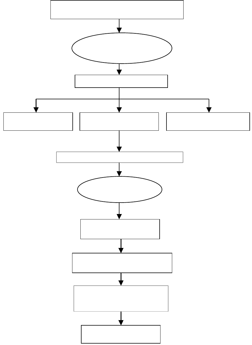
Figure 3.1 Algorithm for the voltage stability analysis.

Obtain the load flow solution for a base case of the

system and get the Jacobian matrix (J)

Compute the eigenvalue of J

R

(

λ

)

If λ

i

< 0

The system is voltage unstable

If

λ

> 0

The system is voltage stable

If λ

i

= 0

The system will collapse

How close is the system to voltage instability?

Find the minimum

eigenvalue of J

R

(λ

min

)

Calculate the right and left

eigenvectors of J

R

(Φ and Γ)

Compute the Participation factor (P

ki

)

for (

λ

min

)

i

:

ikkiki

P ΓΦ=

The highest P

ki

will indicate the

most participated k

th

bus to i

th

mode in the s

y

stem.

Generate the Q-V curve to

the participated k

th

bus.

Compute the reduced Jacobian

matrix (J

R

)

[

]

12

1

112122

JJJJJ

R

−

−=

CHAPTER 3 METHOD OF ANALYSIS

22

3.4 Q-V Curve

V-Q or voltage- reactive power curves are generated by series of power flow simulation. They plot

the voltage at a test bus or critical bus versus reactive power at the same bus. The bus is considered

to be a PV bus, where the reactive output power is plotted versus scheduled voltage. Most of the

time these curves are termed Q-V curves rather than V-Q curves. Scheduling reactive load rather

than voltage produces Q-V curves. These curves are a more general method of assessing voltage

stability. They are used by utilities as a workhorse for voltage stability analysis to determine the

proximity to voltage collapse and to establish system design criteria based on Q and V margins

determined from the curves. Operators may use the curves to check whether the voltage stability of

the system can be maintained or not and take suitable control actions. The sensitivity and variation

of bus voltages with respect to the reactive power injection can be observed clearly. The main

drawback with Q-V curves is that it is generally not known previously at which buses the curves

should be generated.

As a traditional solution in system planning and operation, the voltage level is used as an index of

system voltage instability. If it exceeds the limit, reactive support is installed to improve voltage

profiles. With such action, voltage level can be maintained within acceptable limits under a wide

range of MW loadings. In reality, voltage level may never decline below that limit as the system

approaches its steady state stability limits. Consequently, voltage levels should not be used as a

voltage collapse warning index.

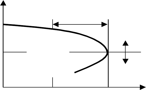
Figure 3.2 shows a typical Q-V curve. The Q axis shows the reactive power that needs to be added

or removed from the bus to maintain a given voltage at a given load. The reactive power margin is

the Mvar distance from the operating point to the bottom of the curve. The curve can be used as an

index for voltage instability (dQ/dV goes negative). Near the nose of a Q-V curve, sensitivities get

very large and then reverse sign. Also, it can be seen that the curve shows two possible values of

CHAPTER 3 METHOD OF ANALYSIS

23

voltage for the same value of power. The power system operated at lower voltage value would

require very high current to produce the power. That is why the bottom portion of the curve is

classified as an unstable region; the system can’t be operated, in steady state, in this region.

Accordingly, any discussion regarding such kind of operation is just educational. The steady state

voltage problem analysis will be focused on the practical range of an operating system; the top

portion of the curve. Hence, the top portion of the curve represents the stability region while the

bottom portion from the stability limit indicates the unstable operating region. It is preferred to

keep the operating point far from the stability limit.

In normal operating condition, an operator will attempt to correct the low voltage condition by

increasing the terminal voltage. However, if the system is operating on the lower portion of the

curve, the unstable region, increasing the terminal voltage will cause an even further drop in the

load voltage; an unstable situation.

The Q-V curves have several advantages [1]:

1. Voltage security is closely related to reactive power, where the reactive power margin for a test

bus can be determined from these curves.

2. Characteristics of test bus shunt reactive compensation (capacitor, SVC or synchronous

condenser) can be plotted directly on the Q-V curve. The operating point is the intersection of

the Q-V system characteristic and the reactive power compensation characteristic. This is

useful since the reactive compensation is often a solution to voltage stability problems.

3. Q-V curves can be computed at points along P-V curve to test system robustness.

4. The slope of the Q-V curve indicates the stiffness of the test bus.

CHAPTER 3 METHOD OF ANALYSIS

24

Mvar distance to

critical point

Operating Point

Q

V

Stability Limit

Stable region

Unstable region

Q

max

Figure 3.2 Typical Q-V curve.

3.5 Effect of Load Modeling

Normally, stability was often regarded as a problem of generators and their controls, while the

effect of loads was considered as a secondary factor. The load representation can play an important

factor in the power system stability. The effects of load characteristics on power system stability

have been studied. Many of research results showed that the load characteristics affect the

behavior of the power system.

The load characteristics can be divided into two categories, static characteristics and dynamic

characteristics. The effect of the static characteristics is discussed in this section [28].

Recently, the load representation has become more important in power system stability studies. In

the previous analysis, the load was represented by considering the active power and reactive

power. Both were represented by combination of constant impedance (resistance or reactance),

constant current and constant power (active or reactive) elements. This kind of load modeling has

been used in many of the power system steady state analyses. However the load may be modeled

as a function of voltage, frequency etc… depending on the type of study. On the other hand, there

is no single load model that leads to conservative design for all system configurations [29].

CHAPTER 3 METHOD OF ANALYSIS

25

The effect of the static load modeling on voltage stability is presented in this section. A voltage

dependent load model is proposed. The new load model is used instead of the constant load used

previously. A significant change in the stability limit or distance to voltage collapse should be

noticed clearly.

3.5.1 Voltage Dependent Load.

Voltage dependency of reactive power affects the steady state stability of power system. This

effect primarily appears on voltages, which in turn affect the active power. It is well known that

the stability improves and the system becomes voltage stable by installing static reactive power

compensators or synchronous condensers [15].

The active and reactive proposed static load model for a particular load bus in this study is an

exponent function of the per unit bus voltage as shown in the following equations:

o

np

k

ok

V

PP

=

3.13

o

nq

k

ok

V

QQ

=

3.14

where:

P

o

= initial bus load active power.

Q

o

= initial bus load reactive power.

Vo = initial bus load voltage.

np = active power voltage exponent.

nq = reactive power voltage exponent.

Then the load flow equation (2.6) at load bus k can be written as:

∑

=

−−+=

n

m

kmmkmkkm

o

np

k

o

VVY

V

P

1

)cos(0

γθθ

3.15

∑

=

−−+=

n

m

kmmkmkkm

o

nq

k

o

VVY

V

Q

1

)sin(0

γθθ

3.16

CHAPTER 3 METHOD OF ANALYSIS

26

Equations (3.15) and (3.16) will update the load equations in the load flow. Then, the nonlinear

equations will be solved to obtain a new load flow solutions. A load flow Matlab based program is

developed to include the proposed load model. After that, the same algorithm used before in figure

3.1 can be followed with the new load flow solution.

3.6 Effect of Induction Motor Load.

Induction machine motor is one of the most popular loads in the power system. About 50-70% of

all generated power is consumed by electric motors with about 90% of this being used by

induction motors [1]. Therefore, it is considered an important part of the power system load and a

significant attention regarding this type of load has been taken for both dynamic and steady state

analysis.

In this research, the induction machine load is considered using the steady state model equivalent

circuit [3] as shown in Figure 3.3

Figure 3.3 Equivalent circuit for steady state operation of a symmetrical induction machine.

The input impedance of the equivalent circuit shown in Figure 3.3 is:

'

lr

b

e

Xj

ω

ls

b

e

Xj

ω

M

b

e

Xj

ω

s

r

V

I

s

r

'

r

CHAPTER 3 METHOD OF ANALYSIS

27

()

'

'2

2

'

rr

b

e

r

rrsss

r

b

e

rrssM

b

ers

Xj

s

r

XrX

s

r

jXXX

s

rr

Z

ω

+













++−













+

= (3.17)

where,

f2

XXX

s

eb

M

'

lr

'

rr

Mlsss

e

re

π=ω=ω

+=

ω

ω−ω

=

s = machine slip.

r

s

= stator resistance.

r

’

= rotor resistance referred to the stator side.

X

ls

= stator leakage inductance.

X

lr

’

= rotor leakage inductance referred to the stator side.

Since,

Z

V

I

→

= (3.18)

Then the power consumed by the induction motor is:

*

→→

=

IVS

(3.19)

QjPS

+= (3.20)

From Equations (3.17) to (3.20), it can be seen that both the active and reactive power consumed

by the induction motor are function of the bus voltage and the machine slip. A load flow program

using Matlab is developed to include the proposed induction machine load model. The algorithm

used before in Figure 3.1 can be followed with the new load flow solution.

CHAPTER 4 RESULTS AND DISCUSSION

28

CHAPTER 4

RESULTS AND DISCUSSION

4.1 Introduction.

The Modal analysis method has been successfully applied to three different electric power

systems. The Q-V cures are generated for selected buses in order to monitor the voltage stability

margin. Different voltage dependent load and Induction machine load models are simulated. A

power flow program based on Matlab is developed to:

1. Calculate the power flow solution.

2. Analyze the voltage stability based on modal analysis.

3. Generate the Q-V curves.

4. Demonstrate the impact of voltage dependent load and Induction machine load models on

the system voltage stability.

4.2 Test Systems Description

Three systems have been simulated and tested in this project to illustrate the proposed analysis

methods:

1. Western System Coordinating Council (WSCC) 3-Machines 9-Bus system. The single line

diagram is shown in Figure 4.1.

2. The IEEE 14 Bus Test Case represents a portion of the American Electric Power System

(in the Midwestern US) . The single line diagram is shown in Figure 4.2.

3. The IEEE 30 Bus Test Case represents a portion of the American Electric Power System

(in the Midwestern US). The single line diagram is shown in Figure 4.3.

CHAPTER 4 RESULTS AND DISCUSSION

29

Figure 4.1 Western System Coordinating Council (WSCC) 3-Machines 9-Bus system.

Figure 4.2 Single line diagram of the IEEE 14 Bus System.

CHAPTER 4 RESULTS AND DISCUSSION

30

Figure 4.3 Single line diagram of the IEEE 30 Bus System.

4.3 Analysis with Constant Impedance Load.

The modal analysis method is applied to the three suggested test systems. The voltage profile of

the buses is presented from the load flow simulation. Then, the minimum eigenvalue of the

reduced Jacobian matrix is calculated. After that, the weakest load buses, which are subject to

voltage collapse, are identified by computing the participating factors. The results are shown in

Figure 4.4 to Figure 4.12.

4.3.1 Western System Coordinating Council (WSCC) 3-Machines 9-Bus system.

Figure 4.4 shows the voltage profile of all buses of the Western System Coordinating Council

(WSCC) 3-Machines 9-Bus system as obtained form the load flow. It can be seen that all the bus

CHAPTER 4 RESULTS AND DISCUSSION

31

voltages are within the acceptable level (± 5%); some standards consider (± 10%). The lowest

voltage compared to the other buses can be noticed in bus number 5.

Voltage Profile of all Buses [3-Machine 9-Bus System]

0.97

0.98

0.99

1

1.01

1.02

1.03

1.04

1.05

123456789

Bus number

Voltage [p.u]

Figure 4.4 Voltage profiles of all buses of the WSCC 3-Machines 9-Bus system.

Since there are nine buses among which there is one swing bus and two PV buses, then the total

number of eigenvalues of the reduced Jacobian matrix

J

R

is expected to be six as shown in

Table4.1. Note that all the eigenvalues are positive which means that the system voltage is stable.

Table 4.1 WSCC 3-Machines 9-Bus system eigenvalues.

# 1 2 3 4 5 6

Eigenvalue 51.0938 5.9589 46.6306 12.9438 14.9108 36.3053

From Table 4.1, it can be noticed that the minimum eigenvalue

λ

= 5.9589 is the most critical

mode. The participating factor for this mode has been calculated and the result is shown in

Figure 4.5. The result shows that, the buses 5,6 and 8 have the highest participation factors to the

CHAPTER 4 RESULTS AND DISCUSSION

32

critical mode. The largest participation factor value (0.3) at bus # 5 indicates the highest

contribution of this bus to the voltage collapse.

Participation Factors for Minimum Eigenvalue (5.9589)

[3-Machine 9-Bus System]

0

0.05

0.1

0.15

0.2

0.25

0.3

0.35

456789

Bus number

Participation Factor

Figure 4.5 The participating factor of all buses for most critical mode for the WSCC 3-Machines 9-Bus

system.

The Q-V curves are used to determine the Mvar distance to the voltage instability point or the

voltage stability margins. The margins were determined between the base case loading points and

the maximum loading points before the voltage collapse. Consequently, these curves can be used

to predict the maximum-security margins that can be reached. In other words, by using Q-V

curves, it is possible for the operators and the planners to know what is the maximum reactive

power that can be achieved or added to the weakest bus before reaching minimum voltage limit or

voltage instability. In addition, the calculated Mvar margins could relate to the size of shunt

capacitor or static var compensation in the load area.

CHAPTER 4 RESULTS AND DISCUSSION

33

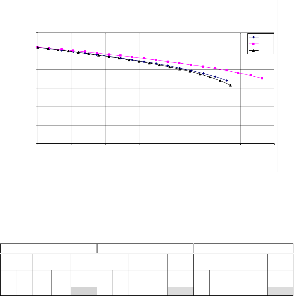
The Q-V curves were computed for the weakest buses of the critical mode in the Western System

Coordinating Council (WSCC) 3-Machines 9-Bus system as expected by the modal analysis

method. The curves are shown in Figure 4.6.

Figure 4.6 The Q-V curves at buses 5, 8 and 6 for the WSCC 3-Machines 9-Bus system.

The Q-V curves shown in figure 4.6 confirm the results obtained previously by the modal analysis

method. It can be seen clearly that bus # 5 is the most critical bus compared with the other buses,

where any more increase in the reactive power demand at that bus will cause a voltage collapse.

Table 4.2 Voltage and reactive power margins for the WSCC 3-Machines 9-Bus system from Q-V curves.

Table 4.2 shows evaluation of the buses 5, 6, and 8 Q-V curves. These results can be used

effectively in planning or operation of this system.

Bus # 5 Bus # 6 Bus # 8

Operating

Point

Maximum

withstand

Stability

Margin

Operating

Point

Maximum

withstand

Stability

Margin

Operating

Point

Maximum

withstand

Stability

Margin

V

(pu)

Q

(pu)

V

(pu)

Q

(pu)

Q (pu) V

(pu)

Q

(pu)

V (pu) Q

(pu)

Q (pu) V

(pu)

Q

(pu)

V (pu) Q

(pu)

Q (pu)

1 0.5 0.724 2.625 2.125 1 0.3 0.6297 2.85 2.55 1 0.35 0.7042 3.325 2.975

Q-V Curve [3-Machine 9-Bus System]

0

0.2

0.4

0.6

0.8

1

1.2

0 0.5 1 1.5 2 2.5 3 3.5

Reactive Power [p.u]

Bus Voltage [p.u]

Bus # 5

Bus # 8

Bus # 6

CHAPTER 4 RESULTS AND DISCUSSION

34

4.3.2 The IEEE 14 Bus system.

Figure 4.7 shows the voltage profile of all buses of the IEEE 14 Bus system as obtained form the

load flow. It can be seen that all the bus voltages are within the acceptable level (± 5%). The

lowest voltage compared to the other buses can be noticed in bus number 4.

Since there are 14 buses among which there is one swing bus and 4 PV buses, then the total

number of eigenvalues of the reduced Jacobian matrix

J

R

is expected to be 9 as shown in table 4.3.

Table 4.3 IEEE 14 Bus system eigenvalues.

# 1 2 3 4 5 6 7 8 9

Eigenvalue 62.5497 40.0075 21.5587 2.7811 11.1479 15.7882 5.4925 18.7197 7.5246

Voltage Profile of all Buses [IEEE 14-Bus System]

0

0.2

0.4

0.6

0.8

1

1.2

1234567891011121314

Bus number

Voltage [p.u]

Figure 4.7 Voltage profiles of all buses of the IEEE 14 Bus system.

Note that all the eigenvalues are positive which means that the system voltage is stable.

CHAPTER 4 RESULTS AND DISCUSSION

35

From Table 4.3, it can be noticed that the minimum eigenvalue λ = 2.7811 is the most critical

mode. The participating factor for this mode has been calculated and the result is shown in

Figure-4.8.

The result shows that, the buses 14, 10 and 9 have the highest participation factors for the critical

mode. The largest participation factor value (0.327) at bus 14 indicates the highest contribution of

this bus to the voltage collapse.

Participation Factors for Minimum Eigenvalue (2.7811)

[IEEE 14-Bus System]

0

0.05

0.1

0.15

0.2

0.25

0.3

0.35

45791011121314

Bus number

Participation Factor

Figure 4.8 The participating factor of all buses for most critical mode for the IEEE 14 Bus system.

The Q-V curves were computed for the weakest buses of the critical mode in the IEEE 14 Bus

system as expected by the modal analysis method. The curves are shown in Figure 4.9.

Figures 4.9, Q-V curves, prove the results obtained previously by modal analysis method. It can be

seen clearly that bus # 14 is the most critical bus compared the other buses, where any more

increase in the reactive power demand in that bus will cause a voltage collapse.

CHAPTER 4 RESULTS AND DISCUSSION

36

Q-V Curve [IEEE 14-Bus System]

0

0.2

0.4

0.6

0.8

1

1.2

00.51 1.5 2 2.5

Reactive Power [p.u]

Bus Voltage [p.u]

Bus # 9

Bus # 10

Bus # 14

Figure 4.9 The Q-V curves at buses 9, 10 and 14 for the IEEE 14 Bus system.

Table 4.4 Voltage and reactive power margins for the IEEE 14 Bus system from Q-V curves.

Bus # 9 Bus # 10 Bus # 14

Operating

Point

Maximum

withstand

Stability

Margin

Operating

Point

Maximum

withstand

Stability

Margin

Operating

Point

Maximum

withstand

Stability

Margin

V

(pu)

Q (pu) V (pu) Q

(pu)

Q (pu) V

(pu)

Q

(pu)

V (pu) Q

(pu)

Q (pu) V

(pu)

Q

(pu)

V (pu) Q

(pu)

Q (pu)

1 -

0.1421

0.6102 2.34 2.4821 1 0.032 0.6521 1.8 1.768 1 0.05 0.6349 1.17 1.12

Table 4.4 shows evaluation of the buses 9, 10, and 14 Q-V curves. These results can be used

effectively in planning or operation of this system.

4.3.3 The IEEE 30 Bus system.

Figure 4.10 shows the voltage profile of all buses of the IEEE 30 Bus system as obtained form the

load flow. It can be seen that all the bus voltages are within the acceptable level (

±

5%) except bus

CHAPTER 4 RESULTS AND DISCUSSION

37

number 30, which is about 0.944 p.u. The lowest voltage compared to the other buses can be

noticed in bus number 30.

Voltage Profile of all Buses [IEEE 30-Bus System]

0.85

0.9

0.95

1

1.05

1.1

123456789101112131415161718192021222324252627282930

Bus number

Voltage [p.u]

Figure 4.10 Voltage profiles of all buses of the IEEE 30 Bus system.

Since there are 30 buses among which there is one swing bus and 5 PV buses, then the total

number of eigenvalues of the reduced Jacobian matrix

J

R

is expected to be 24 as shown in

Table 4.5.

Note that all the eigenvalues are positive which means that the system voltage is stable. From

Table 4.5, it can be noticed that the minimum eigenvalue λ = 0.506 is the most critical mode. The

participating factor for this mode has been calculated and the result is shown in Figure 4.11.

The result shows that, the buses 30, 29 and 26 have the highest participation factors for the critical

mode. The largest participation factor value (0.2118) at bus 30 indicates the highest contribution of

this bus to the voltage collapse.

CHAPTER 4 RESULTS AND DISCUSSION

38

Table 4.5 IEEE 30 Bus system eigenvalues sorted by ascending values.

# Eigenvalue

1 110.2056

2 100.6465

3 65.9541

4 59.5431

5 37.8188

6 35.3863

7 23.0739

8 23.4238

9 19.1258

10 19.7817

11 18.0785

12 16.3753

13 0.506

14 13.7279

15 13.6334

16 1.0238

17 11.0447

18 1.7267

19 8.7857

20 3.5808

21 4.0507

22 7.436

23 6.0207

24 5.4527

The Q-V curves were computed for the weakest buses of the critical mode in the IEEE 30 Bus

system as expected by the modal analysis method. The curves are shown in Figure 4.12.

Figure 4.12, Q-V curves, verifies the results obtained previously by modal analysis method. It can

be seen clearly that bus # 30 is the most critical bus compared the other buses, where any more

increase in the reactive power demand in that bus will cause a voltage collapse.

Table 4.6 Voltage and reactive power margins for the IEEE 30 Bus system from Q-V curves.

Bus # 26 Bus # 29 Bus # 30

Operating

Point

Maximum

withstand

Stability

Margin

Operating

Point

Maximum

withstand

Stability

Margin

Operating

Point

Maximum

withstand

Stability

Margin

V

(pu)

Q

(pu)

V (pu) Q

(pu)

Q (pu) V

(pu)

Q

(pu)

V (pu) Q

(pu)

Q (pu) V

(pu)

Q

(pu)

V (pu) Q

(pu)

Q (pu)

1 0.023 0.5768 0.315 0.292 1 0.009 0.5452 0.36 0.351 1 0.019 0.6688 0.285 0.266

CHAPTER 4 RESULTS AND DISCUSSION

39

Table 4.6 shows evaluation of the buses 30, 29, and 26 Q-V curves. These results can be used

effectively in planning or operation of this system.

Participation Factors for Minimum Eigenvalue (0.5060)

[IEEE 30-Bus System]

0

0.05

0.1

0.15

0.2

0.25

3 4 6 7 9 10121415161718192021222324252627282930

Bus number

Participation Facto

r

Figure 4.11 The participating factor of all buses for most critical mode for the IEEE 30 Bus system.

Figure 4.12 The Q-V curves at buses 30, 29 and 26 for the IEEE 30 Bus system.

Q-V Curve [IEEE 30-Bus System]

0

0.2

0.4

0.6

0.8

1

1.2

0 0.05 0.1 0.15 0.2 0.25 0.3 0.35 0.4

Reactiv e P o w e r [p .u ]

Bus Voltage [

p

Bus # 30

Bus # 29

Bus # 26

CHAPTER 4 RESULTS AND DISCUSSION

40

4.4 Analysis Considering Load Characteristics.

The modal analysis including load characteristics is performed for the three suggested test

systems. Different voltage dependent load models can be implemented by changing the np and nq

values in equations (3.15) and (3.16). The voltage profile of the buses is presented from the load

flow solution. Then, the minimum eigenvalue of the reduced Jacobian matrix is calculated. After

that, computing the participating factors identifies the weakest load buses, which are subject to

voltage collapse. The results are shown in Figure 4.13 to Figure 4.26.

4.4.1 Western System Coordinating Council (WSCC) 3-Machines 9-Bus system.

Figure 4.13 shows the voltage profiles of all buses of the Western System Coordinating Council

(WSCC) 3-Machines 9-Bus system as obtained form the load flow considering different load

characteristics. The result shows four types of loads, including constant load (np = nq = 0 ) and

three different voltage dependent loads (np = nq = 1, np = nq = 2 and np = nq = 3). It can be seen

that all the bus voltages are within the acceptable level (± 5%); some standards consider (± 10%).

In general, the lowest voltage compared to the other buses can be noticed at bus number 5 in all

cases.

Table 4.7 WSCC 3-Machines 9-Bus system eigenvalues at different np and nq values.

λ

at np = nq =

0

λ

at np = nq =

1

λ

at np = nq =

2

λ

at np = nq = 3

1 51.0938 50.8757 50.8106 50.8012

2 5.9589 5.9003 5.8806 5.8778

3 46.6306 46.3852 46.3063 46.2921

4 12.9438 12.7244 12.6545 12.6397

5 14.9108 14.8586 14.8505 14.8531

6 36.3053 36.1263 36.0700 36.0590

Again the total number of eigenvalues of the reduced Jacobian matrix

J

R

is expected to be six as

shown in Table 4.7. The eigenvalues are listed for the all simulated load types. Note that all the

eigenvalues are positive which means that the system voltage is stable.

CHAPTER 4 RESULTS AND DISCUSSION

41

Figure 4.13 Voltage profiles of all buses of the WSCC 3-Machines 9-Bus system at different load models.

Figure 4.14 The participating factor of all buses for most critical modes for the WSCC 3-Machines 9-Bus

system at different load models.

Voltage Profile of all Buses [3-Machine 9-Bus System]

with different Load Characteristics

0.97

0.98

0.99

1

1.01

1.02

1.03

1.04

1.05

123456789

Bus number

Voltage [p.u]

Constant Load

Effect of Non-Linear load [np = nq = 1]

Effect of Non-Linear load [np = nq = 2]

Effect of Non-Linear load [np = nq = 3]

P articip atio n Factors for Minimum Eigenvalue

[3-M ach in e 9-Bus System]

0

0.05

0.1

0.15

0.2

0.25

0.3

0.35

456789

Bus num ber

Participation Facto

r

Constant Load

Effe ct of Non- Linea r load [np = nq = 1]

Effe ct of Non- Linea r load [np = nq = 2]

Effe ct of Non- Linea r load [np = nq = 3]

CHAPTER 4 RESULTS AND DISCUSSION

42

From Table 4.7, it can be noticed that the minimum eigenvalue located in the 2

nd

mode, which is

the most critical mode. The participating factors for these modes have been calculated and the

result is shown in Figure 4.14. In general, the result shows that, the buses 5,6 and 8 have the

highest participation factors to the critical mode, which are similar as obtained before using the

constant load model. The largest participation factor value at bus # 5 indicates a high contribution

of this bus to the voltage collapse especially with constant load and when np =nq =1 for the load

model. However, the situation changes a little bit with the load models np = nq = 2 and np = nq = 3

and bus # 6 appears to be the most critical bus.

The Q-V curves were generated for the weakest buses, bus # 5 and bus # 6, of the critical mode in

the Western System Coordinating Council (WSCC) 3-Machines 9-Bus system as expected by the

modal analysis method at different voltage dependent load models. The curves are shown in Figure

4.15 and Figure 4.16.

Figure 4.15 The Q-V curves at bus 5 for the WSCC 3-Machines 9-Bus system at different load models.

Q -V Curve [3-M achine 9-Bus System ] at Bus # 5

with different Load Characteristics

0.99

0.992

0.994

0.996

0.998

1

1.002

1.004

1.006

1.008

1.01

0 0.5 1 1.5 2 2.5 3 3.5 4

R eactive Power [p.u]

B us Voltage [p.u

V a t np = nq = 1

V a t np = nq = 2

V a t np = nq = 3

CHAPTER 4 RESULTS AND DISCUSSION

43

Figure 4.16 The Q-V curves at bus 6 for the WSCC 3-Machines 9-Bus system at different load models.

Table 4.8 Voltage and reactive power margins for the WSCC system from Q-V curves for bus # 5.

np = nq = 0 np = nq = 1 np = nq = 2 np = nq = 3 Operating

Point

Maximum

withstand

Margin Maximum

withstand

Margin Maximum

withstand

Margin Maximum

withstand

Margin

V Q V Q ∆V ∆Q V Q ∆V ∆Q V Q ∆V ∆Q V Q ∆V ∆Q

1

0.5

0.724

2.625

0.276

2.125

0.9911

3.75

0.0089

3.25

0.9983

3

0.0017

2.5

0.9995

2.7

0.0005

2.2

Table 4.9 Voltage and reactive power margins for the WSCC system from Q-V curves for bus # 6.

np = nq = 0 np = nq = 1 np = nq = 2 np = nq = 3 Operating

Point

Maximum

withstand

Margin Maximum

withstand

Margin Maximum

withstand

Margin Maximum

withstand

Margin

V Q V Q

∆

V

∆

Q V Q

∆

V

∆

Q V Q

∆

V

∆

Q V Q

∆

V

∆

Q

1

0.3

0.6297

2.85

0.3703

2.55

0.9924

3.75

0.0076

3.45

0.9990

3.5

0.0010

3.2

0.9998

3.9

0.0002

3.6

Q-V Curve [3 -M a c h ine 9-Bus System ] at Bus # 6

with diffe re n t Load Characteristics

0.99

0.995

1

1.005

1.01

1.015

0 0.5 1 1.5 2 2.5 3 3.5 4 4.5

Reactive Power [p.u]

Bus Voltage [p.u

V at np = nq = 1

V at np = nq = 2

V at np = nq = 3

CHAPTER 4 RESULTS AND DISCUSSION

44

Figure 4.17 The Q-V curves at bus 5 for the WSCC 3-Machines 9-Bus system at different load models

(Unstable system).

Figure 4.18 The Q-V curves at bus 6 for the WSCC 3-Machines 9-Bus system at different load models

(Unstable system).

Q-V C urve [3-Machine 9-B us S ystem ] at B us # 5 with

different Load C haracteristics [System C ollapse]

0

0.2

0.4

0.6

0.8

1

1.2

0123456

Reactive Power [p.u]

B us Voltage [p.u]

V at np = nq = 1

V at np = nq = 2

V at np = nq = 3

Q-V C urve [3-Machine 9-Bus System] at B us # 6 with

different Load C haracteristics [System C ollapse]

0

0.2

0.4

0.6

0.8

1

1.2

1.4

1.6

0123456

Reactive Power [p.u]

B us Voltage [p.u

]

V at np = nq = 1

V at np = nq = 2

V at np = nq = 3

CHAPTER 4 RESULTS AND DISCUSSION

45

From Table 4.8 and Table 4.9, the voltage dependent load model affected the stability margin.

However, these models didn’t change the location of the weakest buses allocated by the constant

load model. On the other hand a noticed change in the voltage level as well as in the distance to

voltage collapse appeared clearly. The voltage level improved by increasing the value of np and

nq, while the distance to voltage collapse reduced as the value of np and nq increased.

Figure 4.17 and Figure 4.18 show the Q-V curves of bus 5 and bus 6 respectively of the Western

System Coordinating Council (WSCC) 3-Machines 9-Bus system while the stability margins are

exceeded. The curves shows unstable operation and the system has a voltage collapse.

4.4.2 The IEEE 14 Bus system.

Figure 4.19 shows the voltage profiles of all buses of the IEEE 14 Bus system as obtained form the

load flow considering different load characteristics. The result shows four types of loads, including

constant load (np = nq = 0 ) and three different voltage dependent loads (np = nq = 1, np = nq = 2

and np = nq = 3). It can be seen that all the bus’s voltages are within the acceptable voltage level.

The lowest voltage compared to the other buses can be noticed in bus number 4 in all cases.

Table 4.10 IEEE 14 Bus system eigenvalues at different np and nq values.

np = nq = 0 np = nq = 1 np = nq = 2 np = nq = 3

1 62.5497 61.6267 58.5146 57.3693

2 40.0075 39.8004 38.6511 38.3935

3 21.5587 21.1833 20.0812 19.7594

4 2.7811 2.6887 2.4167 2.3092

5 11.1479 10.8571 14.1818 13.8291

6 15.7882 15.3665 9.9570 9.5893

7 5.4925 5.3190 5.1743 5.1691

8 18.7197 18.1899 17.8498 17.8003

9 7.5246 7.3038 7.1718 7.1901

Again the total number of eigenvalues of the reduced Jacobian matrix

J

R

is expected to be nine as

shown in Table 4.10. The eigenvalues are listed for the all simulated load types. Note that all the

eigenvalues are positive which means that the system voltage is stable.

CHAPTER 4 RESULTS AND DISCUSSION

46

Figure 4.19 Voltage profiles of all buses of the IEEE 14 Bus system at different load’s models.

From Table 4.10, it can be noticed that the minimum eigenvalue located in the 4

th

mode, is the

most critical mode. The participating factors for these modes have been calculated and the result

are shown in Figure 4.20. In general, the result shows that, the buses 14,10 and 9 have the highest

participation factors to the critical mode, which are similar as obtained before using the constant

load model. The largest participation factor value at bus # 14 indicates the highest contribution of

this bus to the voltage collapse.

The Q-V curves were generated for the weakest bus, bus # 14, of the critical mode in the IEEE 14-

Bus system identified by the modal analysis method. The curves are shown in Figure 4.21.

From Table 4.11, the voltage dependent load model affected the stability margin. However those

models didn’t change the expected participated weakest buses to the voltage collapse compared to

the constant load model. On the other hand, a noticed change in the voltage level as well as in the

distance to voltage collapse appeared clearly. The voltage level improved by increasing the value

Voltage Profile of all Buses [IEEE 14-Bus System ] with

different Load Characteristics

0

0.2

0.4

0.6

0.8

1

1.2

1234567891011121314

Bus number

Voltage [p.u]

Constant Load

Effect of Non-Linear Load [np = nq = 1]

Effect of Non-Linear Load [np = nq = 2]

Effect of Non-Linear Load [np = nq = 3]

CHAPTER 4 RESULTS AND DISCUSSION

47

of np and nq, while the distance to voltage collapse reduced as the value of np and nq was

increased.

Figure 4.20 The participating factor of all buses for most critical modes for the IEEE 14 Bus system at

different load’s models.

Figure 4.21 The Q-V curves at bus 14 for the IEEE 14 Bus system at different load’s models.

P a rtic ip a tio n Factors fo r Minimum Eigenvalues [IEEE

14-Bus System ] with d iffe re n t Load Characteristics

0

0.05

0.1

0.15

0.2

0.25

0.3

0.35

4 5 7 9 10 11 12 13 14

Bus num ber

Participation Facto

r

Cons ta nt Loa d

E ffe c t of Non- Linear Load [np = nq = 1]

E ffe c t of Non- Linear Load [np = nq = 2]

E ffe c t of Non- Linear Load [np = nq = 3]

Q-V Curve [IEEE 14-Bus System at Bus # 14 with

different Load Characteristics

0.98

0.985

0.99

0.995

1

1.005

1.01

0 0.2 0.4 0.6 0.8 1 1.2 1.4 1.6 1.8 2

Reactive Power [p.u]

Bus Voltage [p.u]

V at np = nq = 1

V at np = nq = 3

CHAPTER 4 RESULTS AND DISCUSSION

48

Table 4.11 Voltage and reactive power margins for the IEEE 14 Bus system from Q-V curves for bus # 14.

np = nq = 0 np = nq = 1 np = nq = 3 Operating Point

Maximum

withstand

Margin Maximum

withstand

Margin Maximum

withstand

Margin

V Q V Q ∆V ∆Q V Q ∆V ∆Q V Q ∆V ∆Q

1 0.05 0.5984 1.2 0.4016 1.15 0.9815 1.805 0.0185 1.755 0.9891 1.53 0.0109 1.48

Figure 4.22 The Q-V curves at bus 14 for the IEEE 14 Bus system at different load models (Unstable

system).

Figure 4.22 shows the Q-V curves of bus number 14 of the IEEE 14 Bus system while the stability

margins is exceeded. The curve demonstrates unstable operation.

4.4.3 The IEEE 30 Bus system.

Figure 4.23 shows the voltage profiles of all buses of the IEEE 30 Bus system as obtained form the

load flow considering different load characteristics. The result shows four types of load; including

constant load (np = nq = 0 ) and three different voltage dependent loads (np = nq = 1, np = nq = 2

Q-V Curve [IEEE 14-Bus System at Bus # 14 with

diffe re n t Load Characteristics [S y s te m Collapse]

0

0.2

0.4

0.6

0.8

1

1.2

1.4

1.6

00.511.522.53

Reactive Power [p.u]

Bus Voltage [p.u]

V at np = nq = 1

V at np = nq = 3

CHAPTER 4 RESULTS AND DISCUSSION

49

and np = nq = 3). It can be seen that all the bus voltages are within the acceptable level. The lowest

voltage compared to the other buses can be noticed in bus number 30 in all cases.

Again the total number of eigenvalues of the reduced Jacobian matrix

J

R

is expected to be 24 as

shown in Table 4.12. The eigenvalues are listed for the all simulated load types. Note that all the

eigenvalues are positive which means that the system voltage is stable.

Table 4.12 IEEE 30 Bus system eigenvalues at different np and nq values.

From Table 4.12, it can be noticed that the minimum eigenvalue located in mode number 13,

which is the most critical mode. The participating factors for these modes have been calculated

and the result is shown in Figure 4.24. In general, the result shows that, the buses 30, 29 and 26

have the highest participation factors for the critical mode, which are similar to obtained before

np = nq = 0 np = nq = 1 np = nq = 2 np = nq = 3

1 110.2056 109.3343 108.9713 108.8641

2 100.6465 98.2252 97.8875 97.9381

3 65.9541 65.2630 64.9428 64.8389

4 59.5431 58.2062 57.9080 57.8431

5 37.8188 36.7889 33.7897 36.7142

6 35.3863 34.3580 36.6533 33.5617

7 23.0739 23.0379 23.0083 23.0114

8 23.4238 22.7018 22.4379 22.3712

9 19.1258 19.4576 19.3834 19.3744

10 19.7817 18.8395 18.7544 18.7458

11 18.0785 17.8041 17.7496 17.7568

12 16.3753 16.2569 16.2474 16.2684

13 0.5060 0.5145 0.5178 0.5207

14 13.7279 0.9988 0.9943 0.9960

15 13.6334 1.7635 1.7800 1.7902

16 1.0238 10.8959 10.8333 10.8170

17 11.0447 3.4832 3.4729 3.4803

18 1.7267 8.5203 3.8759 3.8708

19 8.7857 3.9180 8.4374 8.4306

20 3.5808 7.4443 7.4613 7.4813

21 4.0507 6.1538 13.5159 6.2256

22 7.4360 13.5377 6.1989 13.5359

23 6.0207 5.3471 5.3146 5.3156

24 5.4527 13.2696 13.2050 13.2213

CHAPTER 4 RESULTS AND DISCUSSION

50

using the constant load model. The largest participation factor value at bus # 30 indicates a high

contribution of this bus to the voltage collapse.

Figure 4.23 Voltage profiles of all buses of the IEEE 30 Bus system at different types of load models.

Figure 4.24 The participating factor of all buses for most critical modes for the IEEE 30 Bus at different

types of load models.

Voltage Profile of all Buses [IEEE 30-Bus System]

0.85

0.9

0.95

1

1.05

1.1

1 2 3 4 5 6 7 8 9 101112131415161718192021222324252627282930

Bus number

Voltage [p.u]

Constant Load

Effect of Non-Linear Load [np = nq = 1]

Effect of Non-Linear Load [np = nq = 2]

Effect of Non-Linear Load [np = nq = 3]

P a rtic ip a tio n Factors fo r Minimum Eigenvalue (0 .5060)

[IEEE 30-B us System ]

0

0.05

0.1

0.15

0.2

0.25

3 4 6 7 9 10 12 14 15 16 17 18 19 20 21 22 23 24 25 26 27 28 29 30

Bus num ber

Participation Facto

Cons ta nt Load

Effe ct of Non- Linear Loa d [np = nq = 1]

Effe ct of Non- Linear Loa d [np = nq = 2]

Effe ct of Non- Linear Loa d [np = nq = 3]

CHAPTER 4 RESULTS AND DISCUSSION

51

The Q-V curves were generated for the weakest buses, bus # 30, of the critical mode in the IEEE

30-Bus system as expected by the modal analysis method at different voltage dependent load

models. The curves are shown in Figure 4.25.

Figure 4.25 The Q-V curves at bus 30 for the IEEE 30 Bus system at different types of load.

From Table 4.13, the voltage dependent load model affected the stability margin. However, those

models didn’t change the expected participated weakest buses to the voltage collapse compared to

the constant load model. There was a noticed improvement in the voltage level as the value of np

and nq increased, while the distance to voltage collapse reduced as the value of np and nq

increased.

Table 4.13

Voltage and reactive power margins for the IEEE 30 Bus system from Q-V curves for bus # 30.

np = nq = 0 np = nq = 1 np = nq = 2 np = nq = 3 Operating

Point

Maximum

withstand

Margin Maximum

withstand

Margin Maximum

withstand

Margin Maximum

withstand

Margin

V Q V Q ∆V ∆Q V Q ∆V ∆Q V Q ∆V ∆Q V Q ∆V ∆Q

1

0.019

0.6688

0.285

0.3312

0.266

0.9671

0.33

0.0329

0.311

0.9804

0.3

0.0196

0.281

0.9861

0.28

0.0139

0.261

Q-V Curve [IEEE 30-Bus System at Bus # 30 with

different Load C haracteristics

0.965

0.97

0.975

0.98

0.985

0.99

0 0.05 0.1 0.15 0.2 0.25 0.3 0.35

R eactive Power [p.u]

B us Voltage [p.u]

V at np = nq = 1

V at np = nq = 2

V at np = nq = 3

CHAPTER 4 RESULTS AND DISCUSSION

52

Figure 4.26 The Q-V curves at bus 30 for the IEEE 30 Bus system at different load’s models (Unstable

system).

Figure 4.26 shows the Q-V curves of bus number 30 of the IEEE 30 Bus system while the stability

margins is exceeded. The curve indicates unstable operation.

4.5 Analysis Considering Effect of Induction Machine Load.

The modal analysis including the induction machine load is performed for the three suggested test

systems. The induction machine load can be connected to any bus in the tested system. In this

study two induction machine loads with different ratings have been selected for the analysis. The

machines data are shown in Table 4.14. The voltage profile of the buses is presented from the load

flow solution. Then, the minimum eigenvalue of the reduced Jacobian matrix is calculated. After

that, computing the participating factors identifies the weakest load buses, which are subject to

voltage collapse. Finally, the Q-V curves are generated to specific buses and the results are shown

in Figure 4.27 to Figure 4.38.

Q-V Curve [IEEE 30-Bus System at Bus # 30 with

different Load C haracteristics [System Collapse]

0

0.2

0.4

0.6

0.8

1

1.2

1.4

0 0.1 0.2 0.3 0.4 0.5 0.6 0.7 0.8 0.9 1

Reactive Power [p.u]

B us Voltage [p.u]

V a t np = nq = 1

V a t np = nq = 2

V a t np = nq = 3

CHAPTER 4 RESULTS AND DISCUSSION

53

Table 3.14 Induction machine parameters.

Machine rating

hp volts rpm T

B

N.m

I

B(abc)

amps

r

s

Ω

X

ls

Ω

X

M

Ω

X

’

lr

Ω

r

’

r

Ω

J

kg.m

2

500 2300 1773 1980 93.6 0.262 1.206 54.02 1.206 1.187 11.06

2250 2300 1786 8900 421.2 0.029 0.226 13.04 0.226 0.022 63.87

4.5.1 Western System Coordinating Council (WSCC) 3-Machines 9-Bus system.

Figure 4.27 shows the voltage profiles of all buses of the Western System Coordinating Council

(WSCC) 3-Machines 9-Bus system as obtained form the load flow including induction machine

load at bus # 5. The result shows the effect of both induction machine and the constant loads. It

can be seen that all the bus voltages are within the acceptable level (± 5%). In general, the lowest

voltage compared to the other buses can be noticed at bus number 5 in all cases.

Figure 4.27 Voltage profiles of all buses of the WSCC 3-Machines 9-Bus system including Induction

machine load at bus # 5.

Voltage Profile of all B us es [3-Machine 9-B us S ys tem]

Including Induction Machine L oads at B us # 5

0.95

0.96

0.97

0.98

0.99

1

1.01

1.02

1.03

1.04

1.05

123456789

Bus number

Voltage [p.u]

Constant load

Induction machine load at bus # 5 (IM1)

Induction machine load at bus # 5 (IM2)

CHAPTER 4 RESULTS AND DISCUSSION

54

Again the total number of eigenvalues of the reduced Jacobian matrix J

R

is expected to be six as

shown in Table 4.15. The eigenvalues are listed for the all simulated load types. Note that all the

eigenvalues are positive which means that the system voltage is stable.

Figure 4.28 The participating factor of all buses for the most critical modes for the WSCC 3-Machines 9-

Bus system at different load models at bus # 5.

Table 4.15 WSCC 3-Machines 9-Bus system eigenvalues at different loads in bus # 5.

λ at constant

load

λ using

machine 1

λ using

machine 2

1 51.0938

51.0165 50.7747

2 5.9589

5.9354 5.85

3 46.6306

46.5528 46.3713

4 12.9438

12.9115 12.8651

5 14.9108

14.9426 14.7363

6 36.3053

36.2722 36.1804

From Table 4.15, it can be noticed that the minimum eigenvalue is located in the 2

nd

mode, which

is the most critical mode. The participating factors for these modes have been calculated and the

result is shown in Figure 4.28. In general, the result shows that, the buses 5 and 6 have the highest

Participation Factors for Minimum Eigenvalue [3-Machine 9-

Bus System] Including Induction Machine Loads at Bus # 5

0

0.05

0.1

0.15

0.2

0.25

0.3

0.35

456789

Bus number

Participation Factor

Constant load

Induction machine load at bus # 5 (IM1)

Induction machine load at bus # 5 (IM2)

CHAPTER 4 RESULTS AND DISCUSSION

55

participation factors to the critical mode, which are similar the results obtained before using the

constant load model and voltage dependent loads. The largest participation factor value at bus # 5

indicates a high contribution of this bus to the voltage collapse.

Figure 4.29 The Q-V curves at bus 5 for the WSCC 3-Machines 9-Bus system at different load models at

bus# 5.

The Q-V curves were generated for the weakest bus, bus # 5, of the critical mode in the Western

System Coordinating Council (WSCC) 3-Machines 9-Bus system as expected by the modal

analysis method at different load models at bus # 5. The curves are shown in Figure 4.29.

Table 4.16 Voltage and reactive power margins for the WSCC system from Q-V curves for bus# 5.

Constant Load Induction machine 1 Induction machine 2 Operating

Point

Maximum

withstand

Margin Maximum

withstand

Margin Maximum

withstand

Margin

V Q V Q

∆

V

∆

Q V Q

∆

V

∆

Q V Q

∆

V

∆

Q

1 0.5 0.724 2.625 0.276 2.125 0.5719 3.135 0.4281 2.635 0.5945 3.04 0.4055 2.54

From Table 4.16, the induction machine load model affected the stability margin. However, those

models didn’t change the expected weakest buses for the voltage collapse and agreed with the

Q-V Curve at Bus # 5 [3-Machine 9-Bus S ystem]

Including Induction Machine Loads at Bus # 5

0

0.2

0.4

0.6

0.8

1

1.2

00.511.5 22.533.5

R eactive Power [p.u]

B us Voltage [p.u]

Consta nt loa d

Induction m achine load at bus # 5 (IM1)

Induction m achine load at bus # 5 (IM2)

CHAPTER 4 RESULTS AND DISCUSSION

56

constant load model. On the other hand, a slight change in the voltage level as well as in the

distance to voltage collapse appeared.

Figure 4.30 The Q-V curves of bus # 5 for the WSCC 3-Machines 9-Bus system at different induction

machine load models (Unstable system).

Figure 4.30 show the Q-V curves of bus 5 at the Western System Coordinating Council (WSCC)

3-Machines 9-Bus system considering the effect of induction machine load models while the

stability margins are exceeded. The curves show unstable operation.

4.5.2 The IEEE 14 Bus system.

Figure 4.31 shows the voltage profiles of all buses of the IEEE 14 Bus system as obtained form the

load flow including induction machine load at bus # 14. The result shows the effect of both

induction machine load and the constant load. It can be seen that all the bus voltages are within the

acceptable level. In general, the lowest voltage compared to the other buses can be noticed at bus

number 4 in all cases.

Q-V Curves [3-Machine 9-Bus S ystem] of B us # 5 with

Induction Machine L oads at Bus # 5 [S ystem C ollapse]

0

0.2

0.4

0.6

0.8

1

1.2

1.4

1.6

0123456

Reactive Power [p.u]

Bus Voltage [p.u]

Induction machine load at bus # 5 (IM1)

Induction machine load at bus # 5 (IM2)

CHAPTER 4 RESULTS AND DISCUSSION

57

Figure 4.31 Voltage profiles of all buses of the IEEE 14 Bus system including Induction machine load at

bus # 14.

Again the total number of eigenvalues of the reduced Jacobian matrix J

R

is expected to be nine as

shown in Table 4.17. The eigenvalues are listed for all the simulated load types. Note that all the

eigenvalues are positive which means that the system voltage is stable.

Table 4.17 IEEE 14 Bus system eigenvalues at different loads at bus # 14.

λ

at constant

load

λ

using

machine 1

λ

using

machine 2

1

62.5497

62.7199 62.609

2

40.0075

39.9959 39.6377

3

21.5587

21.5789 21.4679

4

2.7811

2.7714 2.6679

5

11.1479

11.1654 11.097

6

15.7882

15.8279 15.7543

7

5.4925

5.4867 5.3967

8

18.7197

18.7337 18.5763

9

7.5246

7.512 7.3341

From Table 4.17, it can be noticed that the minimum eigenvalue is the 4

th

mode, which is the most

critical mode. The participating factors for these modes have been calculated and the result is

V o lta g e P ro file o f a ll B u s e s [IE E E 1 4 -B u s S y s te m ]

Including Induction M achine Loads at Bus # 14

0

0.2

0.4

0.6

0.8

1

1.2

1234567891011121314

Bus number

Voltage [p.u]

Constant load m ode l

In d u c tion m achine loa d a t bus # 5 ( IM1)

In d u c tion m achine loa d a t bus # 5 ( IM2)

CHAPTER 4 RESULTS AND DISCUSSION

58

shown in Figure 4.32. In general, the result shows that, the buses 14,10 and 9 have the highest

participation factors to the critical mode, which are similar as obtained before using the constant

load model and voltage dependent loads. The largest participation factor value at bus # 14

indicates the highest contribution of this bus to the voltage collapse.

Figure 4.32 The participating factor of all buses for most critical modes for the IEEE 14 Bus System at

different load’s models in bus # 14.

The Q-V curves were generated for the weakest bus, bus # 14, in the IEEE 14-Bus system. The

curves are shown in Figure 4.33.

Table 4.18 Voltage and reactive power margins for the IEEE 14 Bus system from Q-V curves for bus # 14.

Constant Load Induction machine 1 Induction machine 2 Operating

Point

Maximum

withstand

Margin Maximum

withstand

Margin Maximum

withstand

Margin

V Q V Q

∆

V

∆

Q V Q

∆

V

∆

Q V Q

∆

V

∆

Q

1 0.05 0.6349 1.17 0.3651 1.12 0.6373 1.1875 0.3627 1.1375 0.6532 1.0925 0.3468 1.0425

From Table 4.18, the induction machine load model affected the stability margin. However, those

models didn’t change the expected weakest buses for the voltage collapse and agreed with the

Participation Factors for M inim um Eigenvalue [IEEE 14-Bus

System ] Including Induction M achine Loads at Bus # 14

0

0.05

0.1

0.15

0.2

0.25

0.3

0.35

0.4

4 5 7 9 10 11 12 13 14

Bus number

P artic ipation F ac to r

Constant load model

Induction machine load at bus # 5 (IM1)

Induction machine load at bus # 5 (IM2)

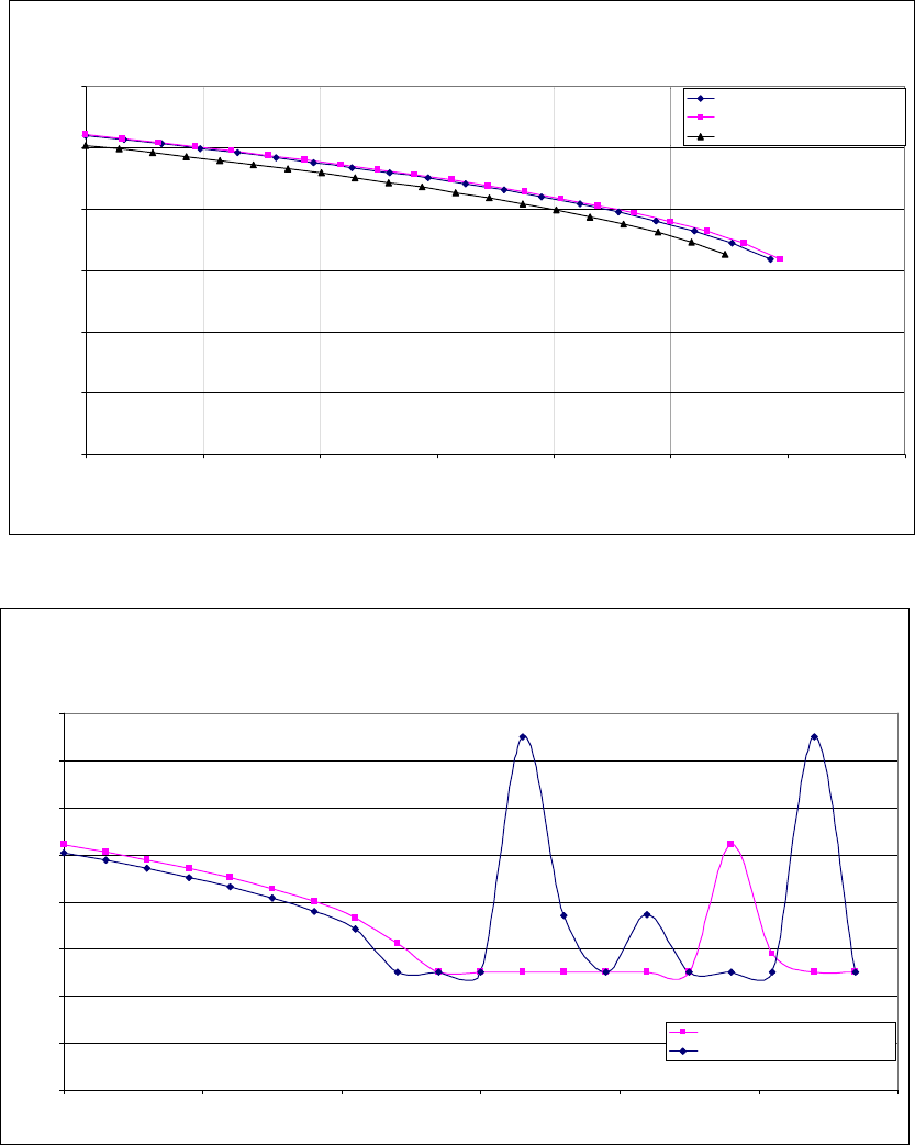
CHAPTER 4 RESULTS AND DISCUSSION

59

results obtained by constant load model and dependent voltage load models. On the other hand, a

noticed change in the voltage level as well as in the distance to voltage collapse appeared clearly.

Figure 4.33 The Q-V curves at bus # 14 for the IEEE 14 Bus System at different load’s models in bus # 14.

Figure 4.34 The Q-V curves of bus # 14 for the IEEE 14 Bus system at different induction machine load’s

models at bus # 14 (Unstable system).

Q -V Curve at Bus # 14 [IEEE 14-Bus System ] Including

Induction M achine Loads at Bus # 14

0

0.2

0.4

0.6

0.8

1

1.2

0 0.2 0.4 0.6 0.8 1 1.2 1.4

Reactive Power [p.u]

B us Voltage [p.u]

Constant load model

Induction machine load at bus # 5 (IM1)

Induction machine load at bus # 5 (IM2)

Q-V Curves [IEEE 14 Bus system] of Bus # 14 with Induction

Machine Loads at Bus # 14 [System Collapse]

0

0.2

0.4

0.6

0.8

1

1.2

1.4

1.6

0 0.5 1 1.5 2 2.5 3

Reactive Power [p.u]

Bus Voltage [p.u]

Induction machine load at bus # 5 (IM1)

Induction machine load at bus # 5 (IM2)

CHAPTER 4 RESULTS AND DISCUSSION

60

Figure 4.34 shows the Q-V curves of bus number 14 of the IEEE 14 Bus system considering the

effect of induction machine load models at bus # 14. While the stability margins are being

exceeded, the curve demonstrates unstable operation.

4.5.3 The IEEE 30 Bus system.

Figure 4.35 shows the voltage profiles of all buses of the IEEE 30 Bus system as obtained form the

load flow including induction machine loads at bus # 30. The result shows the effect of both

induction machines load and the constant load. It can be seen that all the bus voltages are within

the acceptable level except buses 29 and 30. In general, the lowest voltage compared to the other

buses can be noticed at bus number 30 in all cases.

Figure 4.35 Voltage profiles of all buses of the IEEE 30 Bus system including Induction machine load at

bus # 30.

Again the total number of eigenvalues of the reduced Jacobian matrix J

R

is expected to be 24 as

shown in Table 4.19. The eigenvalues are listed for all the simulated load types. Note that all the

eigenvalues are positive which means that the system voltage is stable.

Voltage Profile of all Buses [IEEE 30-Bus System] Including

Induction Machine Loads at Bus # 30

0

0.2

0.4

0.6

0.8

1

1.2

1 2 3 4 5 6 7 8 9 101112131415161718192021222324252627282930

Bus number

Voltage [p.u]

Constant load model

Induction machine load at bus # 5 (IM1)

Induction machine load at bus # 5 (IM2)

CHAPTER 4 RESULTS AND DISCUSSION

61

Table 4.19 IEEE 30 Bus system eigenvalues at different loads at bus # 30.

From Table 4.19, it can be noticed that the minimum eigenvalue is located in modes number 13,

14 and 15, which are the most critical modes. The participating factors for these modes have been

calculated and the results are shown in Figure 4.36. In general, the result shows that, the buses 30,

29 and 26 have the highest participation factors to the critical mode, which are similar to the

results obtained before using the constant load model and voltage dependent loads. The largest

participation factor value at bus # 30 indicates a high contribution of this bus to the voltage

collapse.

λ at constant

load

λ using

machine 1

λ using

machine 2

1

110.2056

110.2649 110.0322

2

100.6465

100.4899 99.775

3

65.9541

65.9984 65.8706

4

59.5431

59.4711 59.1563

5

37.8188

35.3631 37.5844

6

35.3863

37.7779 35.2388

7

23.0739

23.4069 23.297

8

23.4238

23.0806 22.9207

9

19.1258

19.1138 19.0051

10

19.7817

18.0663 19.6983

11 18.0785

16.3282 17.9456

12

16.3753

13.7015 15.935

13

0.5060

13.6141 13.3871

14

13.7279

0.4982 13.5787

15

13.6334

1.0176

0.4293

16

1.0238

11.0536 10.9996

17

11.0447

1.7142 0.9713

18

1.7267

8.7766 1.611

19

8.7857

3.5755 8.7311

20

3.5808

4.0463 3.545

21

4.0507

7.4123 7.1496

22

7.4360

5.4383 4.0233

23

6.0207

5.9895 5.5639

24

5.4527

19.7704 5.195

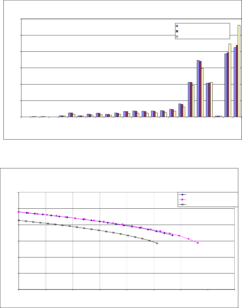
CHAPTER 4 RESULTS AND DISCUSSION

62

The Q-V curves were generated for the weakest buses, bus # 30, of the critical mode in the IEEE

30-Bus system. The curves are shown in Figure 4.37.

Figure 4.36 The participating factor of all buses for most critical modes for the IEEE 30 Bus System at

different load models at bus # 30.

Figure 4.37 The Q-V curves at bus # 30 for the IEEE 30 Bus System at different load’s models in bus # 30.

Q-V Curve at Bus # 30 [IEEE 30-Bus System]

Including Induction Machine Loads at Bus # 30

0

0.2

0.4

0.6

0.8

1

1.2

0 0.05 0.1 0.15 0.2 0.25 0.3 0.35 0.4

Reactive Power [p.u]

Bus Voltage [p.u]

Constant load m ode l

Inductio n m a c h ine load a t bus # 5 ( IM1)

Inductio n m a c h ine load a t bus # 5 ( IM2)

Participation Factors for M inim um Eigenvalue [IEEE 30-Bus

System ] Including Induction M achine Loads at Bus # 30

0

0.05

0.1

0.15

0.2

0.25

0.3

3 4 6 7 9 10 12141516 17181920 21222324 25262728 2930

Bus number

P artic ipation F ac tor

Cons ta nt load m odel

Induction m achine load at bus # 5 (IM 1)

Induction m achine load at bus # 5 (IM 2)

CHAPTER 4 RESULTS AND DISCUSSION

63

Table 4.20 Voltage and reactive power margins for the IEEE 30 Bus system from Q-V curves for bus # 30.

Constant Load Induction machine 1 Induction machine 2 Operating

Point

Maximum

withstand

Margin Maximum

withstand

Margin Maximum

withstand

Margin

V Q V Q

∆

V

∆

Q V Q

∆

V

∆

Q V Q

∆

V

∆

Q

1 0.019 0.6688 0.285 0.3312 0.266 0.5731 0.3325 0.4269 0.3135 0.5693 0.2565 0.4307 0.2375

From Table 4.20, the induction machine load model affected the stability margin. However, those

models didn’t change the expected weakest buses for the voltage collapse and agreed with the

results obtained by constant load model and dependent voltage load models. On the other hand, a

noticed change in the voltage level as well as in the distance to voltage collapse appeared clearly.

Figure 4.38 The Q-V curves of bus # 30 for the IEEE 30 Bus system at different induction machine load

models at bus # 30 (Unstable system).

Figure 4.38 shows the Q-V curves of bus number 30 of the IEEE 30 Bus system. While the

stability margins are exceeded, the curve indicates unstable operation.

Q-V Curves [IEEE 30 Bus system] of Bus # 30 with

Induction Machine Loads at Bus # 30 [System Collapse]

0

0.2

0.4

0.6

0.8

1

1.2

1.4

1.6

0 0.1 0.2 0.3 0.4 0.5 0.6 0.7

Reactive Power [p.u]

Bus Voltage [p.u]

Induction machine load at bus # 5 (IM1)

Induction machine load at bus # 5 (IM2)

CHAPTER 5 CONCLUSION & RECOMMENDATIONS

64

CHAPTER 5

CONCLUSION & RECOMMENDATIONS

5.1 Conclusion

In this research, the voltage collapse problem is studied. The following can be concluded:

1. The Modal analysis technique is applied to investigate the stability of three well-known

power systems. The method computes the smallest eigenvalue and the associated

eigenvectors of the reduced Jacobian matrix using the steady state system model. The

magnitude of the smallest eigenvalue gives us a measure of how close the system is to the

voltage collapse. Then, the participating factor can be used to identify the weakest node or

bus in the system associated to the minimum eigenvalue.

2. The Q-V curves are used successfully to confirm the result obtained by Model analysis

technique, where the same buses are found to be the weakest and contributing to voltage

collapse.

3. Using the Q-V curves, the stability margin or the distance to voltage collapse is identified

based on voltage and reactive power variation. Furthermore, the result can be used to

evaluate the reactive power compensation.

4. The load characteristic is considered in this study. Different voltage dependent load models

are proposed and applied to the analysis.

5. The results obtained by considering the voltage dependent load models confirmed the ones

obtained by using constant load model. In general, results obtained by the constant load

model and the voltage dependent load models, agreed about the weakest buses that

contribute to voltage instability or voltage collapse. However, using voltage dependent load

CHAPTER 5 CONCLUSION & RECOMMENDATIONS

65

models changes the stability margin and the distance to voltage collapse is improved. In

addition, using the voltage dependent load models maintains much better voltage level.

6. The induction machine load model is considered in this study. The model is represented by

active and reactive powers consumed by the induction motor, where both of them are

function of the machine slip, bus voltage and bus angle. Induction machines with two

different ratings are simulated for the analysis.

7. The results obtained by considering the induction machine load model confirmed the

results previously obtained by using constant load model and voltage dependent load

models. In general, the obtained results agreed about the weakest buses that contribute to

voltage instability or voltage collapse. However, considering induction machine load

model changes the stability margin.

5.2 Recommendations for the Future Research.

This research work leads to various promising topics for future investigations. The following

recommendations are made for the future research:

1. Modeling of the other power system devices such as generators and static var

compensators.

2. Consideration of suitable solutions for the voltage collapse problem in the analyzed system.

REFERENCES

66

REFERENCES

[1] C. W. Taylor, "Power System Voltage Stability." New York: MaHraw-Hill, 1994.

[2] Sauer, Peter W. and Pai, M. A. "Power System Dynamics and Stability" New Jersey Prenitice Hall, 1998.

[3] Machowski, Bialek and Bumby "Power System Dynamics and Stability" John Wiley & Sons Ltd, 1997.

[4] Sirisuth, Piya "Voltage Instability analysis using the Sensitivity of Minimum Singular Value of Load Flow

Jacobian" 1993.

[5] Ajjarapu, V. and Lee, B. "Bibliography on Voltage Stability" IEEE Trans. on Power Systems, vol. 13, pp.

115-125, 1998.

[6] C. Counan, M. Trotignon, E. Corride, G. Bortoni, M. Stubbe, and J. Deuse, "Major incidents on the

French electric system- Potentiality and curative measures," IEEE Trans. on Power Systems, vol. 8, pp.

879-886, Aug. 1993.

[7] R. DÕAquila, N. W. Miller, K. M. Jimma, M. T. Shehan, and G. L. Comegys, "Voltage stability of the

Puget Sound System under Abnormally Cold Weather Conditions," IEEE Trans. on Power Systems, vol. 8,

pp. 1133-1142, Aug. 1993.

[8] F. D. Galiana and Z. C. Zeng, "Analysis of the Load Behavior near Jacobian Singularity," IEEE Trans. on

Power Systems, vol. 7, pp. 1529-1542, Nov. 1992.

[9] P. Kessel and H. Glavitsch, "Estimating the Voltage Stability of a Power System," IEEE Trans. on Power

Delivery, vol. 1, pp. 346-353, July 1986.

[10] Y. Tamura, H. Mori, and S. Iwamoto, "Relationship between Voltage Stability and Multiple Load Flow

Solutions in Electric Systems," IEEE Trans. on Power Apparatus and Systems, vol. PAS-102, pp. 1115-

1123, May 1983.

[11] P. A. Lof, T. Smed, C. Anderson, and D. J. Hill, "Fast Calculation of a Voltage Stability Index," IEEE

Trans. on Power Systems, vol. 7, pp. -64, Feb. 1992.

[12] V. A. Venikov, V. A. Stroev, V. I. Idelchick, and V. I. Trasov, "Estimation of Electric Power System Steady-

State Stability in Load Flow Calculation," IEEE Trans. on Power Apparatus and Systems, vol. PAS-94,

pp. 1034-1041, May/June 1975.

[13] H. G. Kwanti, A. K. Pasrija, and L. Y. Bahar, "Static Bifurcations in Electric Power Networks: Loss of

Steady-State Stability and Voltage Collapse," IEEE Trans. on Circuits and Systems, vol. CAS-33, pp. 981-

991, Oct. 1986.

[14] M. M. Begovic and A. G. Phadke, "Voltage Stability Assessment through measurement of a reduced state

vector," IEEE Trans. on Power Systems, vol. 5, pp. 198-203, Feb. 1990.

[15] P. Pal, "Voltage Stability Conditions Considering Load Characteristics", IEEE Trans. on Power Systems,

Vol. 7, No. 2, pp. 243-249, Feb. 1992.

[16] M. Suzuki, S. Wada, T. Asano, and K. Kudo, "Newly Developed Voltage Security Monitoring System",

IEEE Trans. On Power System, Vol. 7, No. 3, pp. 965-972, August 1992.

[17] Y. Mansour, W. Xu, F. Alverado, and C. Rinzin, "SVC Placement Using Critical Modes of Voltage

Instability", IEEE Trans. On Power Systems, Vol. 9, No. 2, pp. 757-763, May 1994.

[18] E. Vaahedi et al., “Voltage Stability Contingency Screening and Ranking", IEEE Trans. On Power Systems

Vol. 14, No. 1, pp. 256-265 Feb. 1999.

[19] R. Schlueter, "A Voltage Stability Security Assessment Method", IEEE Trans. On Power Systems, Vol. 13,

No. 4, pp. 1423-1438, Nov. 1998.

[20] B. Gao, G. Morison, and P. Kundur, "Voltage Stability Evaluation Using Modal Analysis", IEEE Trans. on

Power Systems, Vol. 7, No. 4, pp. 1423-1543, Nov 1992.

[21] G. Morison, B. Gao and P. Kundur, "Voltage Stability Analysis Using Static and Dynamic Approaches",

IEEE Trans. on Power Systems, Vol. 8, No. 3, pp. 1159-1171, Aug. 1993.

[22] P. A. Lof, G. Anderson, and D. J. Hill, "Voltage Stability Indices For Stressed Power System," IEEE Trans.

on Power Systems, vol. 8, pp. 326-335, Feb. 1993.

[23] N. Flatabo and H. Dommel, "Voltage Stability Condition in a Power Transmission System calculated by

Sensitivity Methods", EEE Trans. on Power Systems, vol. 5, pp. 1286-1293, Nov. 1990.

[24] T. Overbye and C. DeMarco, "Improved Power System stability Assessment Using Energy Method", IEEE

Trans. On Power System, Vol. 6, No. 4, pp. 1890-1896, Nov. 1995.

[25] C. DeMarco and T. Overbye, "An Energy based security Measure for Assessing Vulnerability To Voltage

Collapse", IEEE Trans. On Power System, Vol. 5, No. 2, pp. 419-427, May 1990.

REFERENCES

67

[26] A. El-Keib and X. Ma, "Application of Artificial Neural Networks In Voltage Stability Assessment", IEEE

Trans. On Power System, Vol. 10, No. 4, pp. 1890-1896, Nov. 1995.

[27] C. Liu, C. Chang, and M. Su, "Neuro-Fuzzy Networks for Voltage Security Monitoring based On

Synchronous Pharos Measurements", IEEE Trans.On Power System,Vol. 13, No. 2, May 1998.

[28] Conoordia, C. and Ihara, S., "Load Representation in Power System Stability Studies", IEEE Trans. On

Power Apparatus and Systems Vol. PAS-101, No. 4, pp. 969-976, April. 1982.

[29] Price, William W., Wirgau, Kim A., Murdoch, Alexander, Mitsche, James V., Vaahedi, Ebrahim and El-

Kady, Moe A., "Load Modeling for Power Flow and Transient Stability Computer Studies", IEEE Trans. On

Power Systems Vol. 3, No. No. 1, pp. 180-187, Feb. 1988.

[30] T. Cutsem, "A Method to Compute Reactive Power margins with respect to Voltage", IEEE Trans. On Power

Systems, Vol. PWRS-6, No. 2, pp. 145-156, Feb. 1991

[31] G. Verghes, I. Perez-Arriaga and F. Schewwppe, "Selective Modal Analysis With Application To Electric

Power systems", Part II IEEE trans, I. On Power APP. And System, Vol. PAS 101, No. 9, pp. 3117-

3134, 1982.

[32] E. Vaahedi, Y. Mansour and D. Sun, "Large Scale Voltage Stability Constrained Optimal Planning and

Voltage Stability Applications Using Existing OPF/Optimal Var Planning Tools", IEEE Trans. On Power

Systems Vol. 14, No. 1, Feb.1999.

[33] H. D. Chiang, I. Dobson, R. J. Thomas, J. S. Thorp, and L. Fekih-Ahmed, “ On voltage collapse in

electric power systems” IEEE Trans. on Power Systems, vol. 5, pp. 601-611, May 1990.

[34] J. C. Chow, R. Fischl, and H. Yan, ” on the evaluation of voltage collapse criteria“ IEEE Trans. On Power

Systems, vol. 5, pp. 612-620, May 1990.

[35] C. Barbier and J. P. Barret, "Analysis of Phenomena of Voltage Collapse on a Transmission system," Review

Generale de lÕelectricite, vol. 89, pp. 672-690, Oct. 1980.

[36] R. J. Thomas and A. Tiranuchit, "Voltage Instabilities in Electric Power Networks," Proc. Eighteenth

Southeast Symposium on Systems Theory, pp. 359-363, 1986.

APPENDIX A

68

APPENDIX A

A.1 Test Systems Load Flow Data.

A.1.1 WSCC system Load Flow Data.

This File was Generated: 2000

Western System Coordinating Council (WSCC) 3-Machines 9-Bus system

Bus data format

bus: number,voltage(pu),angle(degree),p_gen(pu),q_gen(pu),

p_load(pu), q_load(pu), conductance(pu), susceptance(pu),

bus_type - 1, swing bus

- 2, generator bus (PV bus)

- 3, load bus (PQ bus)

# V (p.u) δ° P

g

(p.u) Q

g

(p.u) P

L

(p.u) Q

L

(p.u) Condu. Sus. B

Type

1 1.04 0 0.000 0.000 0.000 0.000 0 0 1

2 1.02533 0 1.630 0.000 0.000 0.000 0 0 2

3 1.02536 0 0.850 0.000 0.000 0.000 0 0 2

4 1 0 0.000 0.000 0.000 0.000 0 0 3

5 1 0 0.000 0.000 1.250 0.500 0 0 3

6 1 0 0.000 0.000 0.900 0.300 0 0 3

7 1 0 0.000 0.000 0.000 0.000 0 0 3

8 1 0 0.000 0.000 1.000 0.350 0 0 3

9 1 0 0.000 0.000 0.000 0.000 0 0 3

Line data format

line: from bus, to bus, resistance(pu), reactance(pu),

line charging(pu), tap ratio, phase shift(deg)

From To R (p.u) X (p.u) Line Cha. Tap Phase

2 7 0.0000 0.0625 0.0000 1.00 0.00

7 8 0.0085 0.0720 0.0745*2 1.00 0.00

7 5 0.0320 0.1610 0.1530*2 1.00 0.00

5 4 0.0100 0.0850 0.0880*2 1.00 0.00

4 1 0.0000 0.0576 0.0000 1.00 0.00

4 6 0.0170 0.0920 0.0790*2 1.00 0.00

6 9 0.0390 0.1700 0.1790*2 1.00 0.00

9 3 0.0000 0.0586 0.0000 1.00 0.00

9 8 0.0119 0.1008 0.1045*2 1.00 0.00

tol = 1e-9; % tolerance for convergence

iter

max

= 30; % maximum number of iterations

V

min

= 0.5; % voltage minimum

V

max

= 1.5; % voltage maximum

acc = 1.0; % acceleration factor

APPENDIX A

69

A.1.2 IEEE 14 Bus System Load Flow Data.

This File was Generated: 2000

IEEE 14 bus system

Bus data format

bus: number,voltage(pu),angle(degree),p_gen(pu),q_gen(pu),

p_load(pu), q_load(pu), conductance(pu), susceptance(pu),

bus_type - 1, swing bus

- 2, generator bus (PV bus)

- 3, load bus (PQ bus)

# V (p.u) δ° P

g

(p.u) Q

g

(p.u) P

L

(p.u) Q

L

(p.u) Condu. Sus. B

Type

1 1.06 0 1.4023 0.4443 0.0000 0.0000 0 0 1

2 1.04 0 0.8039 0.2798 0.2170 0.1270 0 0 2

3 1.010 0 1.0445 0.0000 0.9420 0.1900 0 0 2

4 1 0 0.0000 0.0000 0.9670 0.3383 0 0 3

5 1 0 0.0000 0.0000 0.0486 0.3920 0 0 3

6 1.070 0 0.1007 0.4919 0.1120 0.0750 0 0 2

7 1 0 0.0000 0.0000 0.0000 0.0000 0 0 3

8 1.08 0 0.0011 0.1557 0.0000 0.0000 0 0 2

9 1 0 0.0000 0.0000 0.3391 -0.1421 0 0 3

10 1 0 0.0000 0.0000 0.0586 0.0320 0 0 3

11 1 0 0.0000 0.0000 0.0196 0.0280 0 0 3

12 1 0 0.0000 0.0000 0.3674 0.0271 0 0 3

13 1 0 0.0000 0.0000 0.1350 0.0580 0 0 3

14 1 0 0.0000 0.0000 0.1490 0.0500 0 0 3

Line data format

line: from bus, to bus, resistance(pu), reactance(pu),

line charging(pu), tap ratio, phase shift(deg)

From To R (p.u) X (p.u) Line Cha. Tap Phase

1 2 0.01938 0.05917 0.02640 1.00 0.00

2 3 0.04699 0.19797 0.02190 1.00 0.00

2 4 0.05811 0.17632 0.01870 1.00 0.00

1 5 0.05403 0.22304 0.02460 1.00 0.00

2 5 0.05695 0.17388 0.01700 1.00 0.00

3 4 0.06701 0.17103 0.01730 1.00 0.00

4 5 0.01335 0.04211 0.00640 1.00 0.00

5 6 0.00000 0.25202 0.00000 0.932 0.00

4 7 0.00000 0.20912 0.00000 0.978 0.00

7 8 0.00000 0.17615 0.00000 1.00 0.00

4 9 0.00000 0.55618 0.00000 0.969 0.00

7 9 0.00000 0.11001 0.00000 1.00 0.00

9 10 0.03181 0.08450 0.00000 1.00 0.00

6 11 0.09489 0.19891 0.00000 1.00 0.00

6 12 0.12291 0.25581 0.00000 1.00 0.00

6 13 0.06615 0.13027 0.00000 1.00 0.00

9 14 0.12711 0.27038 0.00000 1.00 0.00

10 11 0.08205 0.19207 0.00000 1.00 0.00

12 13 0.22092 0.19988 0.00000 1.00 0.00

13 14 0.17093 0.34802 0.00000 1.00 0.00;

tol = 1e-9; % tolerance for convergence

iter

max

= 30; % maximum number of iterations

V

min

= 0.5; % voltage minimum

V

max

= 1.5; % voltage maximum

acc = 1.0; % acceleration factor

APPENDIX A

70

A.1.3 IEEE 30 Bus System Load Flow Data.

This File was Generated: 1999

IEEE 30 bus system

Bus data format

bus: number,voltage(pu),angle(degree),p_gen(pu),q_gen(pu),

p_load(pu), q_load(pu), conductance(pu), susceptance(pu),

bus_type - 1, swing bus

- 2, generator bus (PV bus)

- 3, load bus (PQ bus)

# V (p.u) δ° P

g

(p.u) Q

g

(p.u) P

L

(p.u) Q

L

(p.u) Condu. Sus. B

Type

1 1.06 0 0 0 0.000 0.000 0 0 1

2 1.043 0 0.4 0 0.217 0.127 0 0 2

3 1 0 0 0 0.024 0.012 0 0 3

4 1 0 0 0 0.076 0.016 0 0 3

5 1.01 0 0 0 0.942 0.190 0 0 2

6 1 0 0 0 0.000 0.000 0 0 3

7 1 0 0 0 0.228 0.109 0 0 3

8 1.01 0 0 0 0.300 0.300 0 0 2

9 1 0 0 0 0.000 0.000 0 0 3

10 1 0 0 0 0.058 0.020 0 0.19 3

11 1.082 0 0 0 0.000 0.000 0 0 2

12 1 0 0 0 0.112 0.075 0 0 3

13 1.071 0 0 0 0.000 0.000 0 0 2

14 1 0 0 0 0.062 0.016 0 0 3

15 1 0 0 0 0.082 0.025 0 0 3

16 1 0 0 0 0.035 0.018 0 0 3

17 1 0 0 0 0.090 0.058 0 0 3

18 1 0 0 0 0.032 0.009 0 0 3

19 1 0 0 0 0.095 0.034 0 0 3

20 1 0 0 0 0.022 0.007 0 0 3

21 1 0 0 0 0.175 0.112 0 0 3

22 1 0 0 0 0.000 0.000 0 0 3

23 1 0 0 0 0.032 0.016 0 0 3

24 1 0 0 0 0.087 0.067 0 0.043 3

25 1 0 0 0 0.000 0.000 0 0 3

26 1 0 0 0 0.035 0.023 0 0 3

27 1 0 0 0 0.000 0.000 0 0 3

28 1 0 0 0 0.000 0.000 0 0 3

29 1 0 0 0 0.024 0.009 0 0 3

30 1 0 0 0 0.106 0.019 0 0 3

Line data format

line: from bus, to bus, resistance(pu), reactance(pu),

line charging(pu), tap ratio, phase shift(deg)

From To R (p.u) X (p.u) Line Cha. Tap Phase

1 2 0.019200 0.057500 0.026400 1.00 0.00

1 3 0.045200 0.185200 0.020400 1.00 0.00

2 4 0.013200 0.037900 0.004200 1.00 0.00

2 5 0.047200 0.198300 0.020900 1.00 0.00

2 6 0.058100 0.176300 0.018700 1.00 0.00

4 6 0.011900 0.041400 0.004500 1.00 0.00

APPENDIX A

71

From To R (p.u) X (p.u) Line Cha. Tap Phase

5 7 0.046000 0.116000 0.010200 1.00 0.00

6 7 0.026700 0.082000 0.008500 1.00 0.00

6 8 0.012000 0.042000 0.004500 1.00 0.00

6 9 0.000000 0.208000 0.000000 0.978 0.00

6 10 0.000000 0.556000 0.000000 0.969 0.00

9 11 0.000000 0.208000 0.000000 1.00 0.00

9 10 0.000000 0.110000 0.000000 1.00 0.00

4 12 0.000000 0.256000 0.000000 0.932 0.00

12 13 0.000000 0.140000 0.000000 1.00 0.00

12 14 0.123100 0.255900 0.000000 1.00 0.00

12 15 0.066200 0.130400 0.000000 1.00 0.00

12 16 0.094500 0.198700 0.000000 1.00 0.00

14 15 0.221000 0.199700 0.000000 1.00 0.00

16 17 0.082400 0.192300 0.000000 1.00 0.00

15 18 0.107000 0.218500 0.000000 1.00 0.00

18 19 0.063900 0.129200 0.000000 1.00 0.00

19 20 0.034000 0.068000 0.000000 1.00 0.00

10 20 0.093600 0.209000 0.000000 1.00 0.00

10 17 0.032400 0.084500 0.000000 1.00 0.00

10 21 0.034800 0.074900 0.000000 1.00 0.00

10 22 0.072700 0.149900 0.000000 1.00 0.00

21 22 0.011600 0.023600 0.000000 1.00 0.00

15 23 0.100000 0.202000 0.000000 1.00 0.00

22 24 0.115000 0.179000 0.000000 1.00 0.00

23 24 0.132000 0.270000 0.000000 1.00 0.00

24 25 0.188500 0.329200 0.000000 1.00 0.00

25 26 0.254400 0.380000 0.000000 1.00 0.00

25 27 0.109300 0.208700 0.000000 1.00 0.00

27 28 0.000000 0.396000 0.000000 0.968 0.00

27 29 0.219800 0.415300 0.000000 1.00 0.00

27 30 0.320200 0.602700 0.000000 1.00 0.00

29 30 0.239900 0.453300 0.000000 1.00 0.00

8 28 0.063600 0.200000 0.021400 1.00 0.00

6 28 0.016900 0.059900 0.006500 1.00 0.00

tol = 1e-9; % tolerance for convergence

iter

max

= 30; % maximum number of iterations

V

min

= 0.5; % voltage minimum

V

max

= 1.5; % voltage maximum

acc = 1.0; % acceleration factor

APPENDIX A

72

A.2 Load Flow Solution.

A.2.1 WSCC system Load Flow Solution with Constant Load Model.

LOAD-FLOW STUDY

REPORT OF POWER FLOW CALCULATIONS

07-Sep-2000

DATA FILE NAME: sys9b3mn.m

SWING BUS : BUS 1

NUMBER OF ITERATIONS : 5

SOLUTION TIME : 0.16 sec.

TOTAL TIME : 0.381 sec.

TOTAL REAL POWER LOSSES : 0.0463789.

TOTAL REACTIVE POWER LOSSES: -0.922664.

GENERATION LOAD

BUS VOLTS ANGLE REAL REACTIVE REAL REACTIVE

1 1.040 0.000 0.716 0.268 0.000 0.000

2 1.025 9.272 1.630 0.067 0.000 0.000

3 1.025 4.659 0.850 -0.108 0.000 0.000

4 1.026 -2.216 0.000 0.000 0.000 0.000

5 0.996 -3.988 0.000 0.000 1.250 0.500

6 1.013 -3.687 0.000 0.000 0.900 0.300

7 1.026 3.715 0.000 0.000 -0.000 -0.000

8 1.016 0.724 0.000 0.000 1.000 0.350

9 1.033 1.962 0.000 0.000 -0.000 -0.000

LINE FLOWS

LINE FROM BUS TO BUS REAL REACTIVE

1 2 7 1.630 0.067

1 7 2 -1.630 0.091

2 7 8 0.764 -0.008

2 8 7 -0.759 -0.107

3 7 5 0.866 -0.083

3 5 7 -0.843 -0.114

4 5 4 -0.407 -0.386

4 4 5 0.409 0.228

5 4 1 -0.716 -0.237

5 1 4 0.716 0.268

6 4 6 0.307 0.009

6 6 4 -0.305 -0.165

7 6 9 -0.595 -0.135

7 9 6 0.608 -0.180

8 9 3 -0.850 0.149

8 3 9 0.850 -0.108

9 9 8 0.242 0.031

9 8 9 -0.241 -0.243

APPENDIX A

73

A.2.2 IEEE 14 Bus System Load Flow Solution with Constant Load Model.

LOAD-FLOW STUDY

REPORT OF POWER FLOW CALCULATIONS

07-Sep-2000

DATA FILE NAME: amer_ieee14n.m

SWING BUS : BUS 1

NUMBER OF ITERATIONS : 5

SOLUTION TIME : 0.13 sec.

TOTAL TIME : 0.401 sec.

TOTAL REAL POWER LOSSES : 0.111425.

TOTAL REACTIVE POWER LOSSES: 0.351199.

GENERATION LOAD

BUS VOLTS ANGLE REAL REACTIVE REAL REACTIVE

1 1.060 0.000 1.517 0.308 0.000 0.000

2 1.040 -2.592 0.804 0.488 0.217 0.127

3 1.010 -5.150 1.045 0.133 0.942 0.190

4 0.979 -8.522 0.000 0.000 0.967 0.338

5 0.983 -7.188 0.000 0.000 0.049 0.392

6 1.070 -14.551 0.101 0.388 0.112 0.075

7 1.046 -12.332 0.000 0.000 -0.000 -0.000

8 1.080 -12.322 0.001 0.209 0.000 0.000

9 1.050 -14.249 0.000 0.000 0.339 -0.142

10 1.049 -14.473 0.000 0.000 0.059 0.032

11 1.056 -14.534 0.000 0.000 0.020 0.028

12 1.024 -17.614 0.000 0.000 0.367 0.027

13 1.044 -16.094 0.000 0.000 0.135 0.058

14 1.029 -16.062 0.000 0.000 0.149 0.050

LINE FLOWS

LINE FROM BUS TO BUS REAL REACTIVE

1 1 2 0.872 0.077

1 2 1 -0.859 -0.065

2 2 3 0.261 0.089

2 3 2 -0.257 -0.098

3 2 4 0.654 0.163

3 4 2 -0.629 -0.108

4 1 5 0.644 0.231

4 5 1 -0.621 -0.162

5 2 5 0.531 0.174

5 5 2 -0.515 -0.141

6 3 4 0.360 0.041

6 4 3 -0.351 -0.036

7 4 5 -0.510 0.069

7 5 4 0.513 -0.064

8 5 6 0.574 -0.025

8 6 5 -0.574 0.100

9 4 7 0.333 -0.202

9 7 4 -0.333 0.234

10 7 8 -0.001 -0.202

10 8 7 0.001 0.209

11 4 9 0.190 -0.062

11 9 4 -0.190 0.083

APPENDIX A

74

12 7 9 0.334 -0.031

12 9 7 -0.334 0.043

13 9 10 0.050 -0.003

13 10 9 -0.050 0.003

14 6 11 0.029 0.064

14 11 6 -0.028 -0.063

15 6 12 0.263 0.070

15 12 6 -0.255 -0.054

16 6 13 0.271 0.079

16 13 6 -0.267 -0.070

17 9 14 0.135 0.019

17 14 9 -0.133 -0.014

18 10 11 -0.009 -0.035

18 11 10 0.009 0.035

19 12 13 -0.113 0.027

19 13 12 0.115 -0.024

20 13 14 0.016 0.036

20 14 13 -0.016 -0.036

A.2.3 IEEE 30 Bus System Load Flow Solution with Constant Load Model.

LOAD-FLOW STUDY

REPORT OF POWER FLOW CALCULATIONS

07-Sep-2000

DATA FILE NAME: amer_ieee30.m

SWING BUS : BUS 1

NUMBER OF ITERATIONS : 5

SOLUTION TIME : 0.17 sec.

TOTAL TIME : 0.33 sec.

TOTAL REAL POWER LOSSES : 0.179697.

TOTAL REACTIVE POWER LOSSES: 0.527394.

GENERATION LOAD

BUS VOLTS ANGLE REAL REACTIVE REAL REACTIVE

1 1.060 0.000 2.614 -0.130 0.000 0.000

2 1.043 -5.509 0.400 0.568 0.217 0.127

3 1.019 -7.987 0.000 0.000 0.024 0.012

4 1.010 -9.651 0.000 0.000 0.076 0.016

5 1.010 -14.414 0.000 0.394 0.942 0.190

6 1.009 -11.378 0.000 0.000 0.000 -0.000

7 1.001 -13.144 0.000 0.000 0.228 0.109

8 1.010 -12.135 0.000 0.404 0.300 0.300

9 1.048 -14.522 0.000 0.000 -0.000 -0.000

10 1.040 -16.172 0.000 0.000 0.058 0.020

11 1.082 -14.522 -0.000 0.177 0.000 0.000

12 1.054 -15.438 0.000 0.000 0.112 0.075

13 1.071 -15.438 -0.000 0.127 0.000 0.000

14 1.038 -16.337 0.000 0.000 0.062 0.016

15 1.033 -16.406 0.000 0.000 0.082 0.025

16 1.041 -16.022 0.000 0.000 0.035 0.018

17 1.035 -16.336 0.000 0.000 0.090 0.058

18 1.023 -17.025 0.000 0.000 0.032 0.009

APPENDIX A

75

19 1.020 -17.200 0.000 0.000 0.095 0.034

20 1.024 -17.001 0.000 0.000 0.022 0.007

21 1.025 -16.616 0.000 0.000 0.175 0.112

22 1.025 -16.600 0.000 0.000 -0.000 -0.000

23 1.018 -16.767 0.000 0.000 0.032 0.016

24 1.006 -16.901 0.000 0.000 0.087 0.067

25 0.983 -16.279 0.000 0.000 0.000 -0.000

26 0.964 -16.729 0.000 0.000 0.035 0.023

27 0.977 -15.626 0.000 0.000 -0.000 0.000

28 1.008 -11.984 0.000 0.000 -0.000 -0.000

29 0.956 -16.978 0.000 0.000 0.024 0.009

30 0.944 -17.951 0.000 0.000 0.106 0.019

LINE FLOWS

LINE FROM BUS TO BUS REAL REACTIVE

1 1 2 1.782 -0.208

1 2 1 -1.727 0.343

2 1 3 0.832 0.078

2 3 1 -0.804 0.016

3 2 4 0.459 0.053

3 4 2 -0.448 -0.038

4 3 4 0.780 -0.028

4 4 3 -0.772 0.045

5 2 5 0.832 0.028

5 5 2 -0.802 0.076

6 2 6 0.619 0.017

6 6 2 -0.599 0.026

7 4 6 0.694 -0.171

7 6 4 -0.688 0.187

8 5 7 -0.140 0.128

8 7 5 0.142 -0.134

9 6 7 0.374 -0.023

9 7 6 -0.370 0.025

10 6 8 0.292 -0.102

10 8 6 -0.291 0.101

11 6 9 0.285 -0.071

11 9 6 -0.285 0.088

12 6 10 0.163 0.011

12 10 6 -0.163 0.003

13 9 11 0.000 -0.172

13 11 9 -0.000 0.177

14 9 10 0.285 0.084

14 10 9 -0.285 -0.075

15 4 12 0.450 0.147

15 12 4 -0.450 -0.098

16 12 13 0.000 -0.125

16 13 12 -0.000 0.127

17 12 14 0.081 0.028

17 14 12 -0.080 -0.026

18 12 15 0.184 0.084

18 15 12 -0.181 -0.079

19 12 16 0.074 0.037

19 16 12 -0.073 -0.036

20 14 15 0.018 0.010

20 15 14 -0.018 -0.010

21 16 17 0.038 0.018

21 17 16 -0.038 -0.017

22 15 18 0.060 0.017

APPENDIX A

76

22 18 15 -0.060 -0.016

23 18 19 0.028 0.007

23 19 18 -0.028 -0.007

24 19 20 -0.067 -0.027

24 20 19 0.067 0.028

25 10 20 0.090 0.036

25 20 10 -0.089 -0.035

26 10 17 0.052 0.041

26 17 10 -0.052 -0.041

27 10 21 0.166 0.120

27 21 10 -0.165 -0.117

28 10 22 0.082 0.059

28 22 10 -0.081 -0.058

29 21 22 -0.010 0.005

29 22 21 0.010 -0.005

30 15 23 0.056 0.048

30 23 15 -0.056 -0.047

31 22 24 0.071 0.063

31 24 22 -0.070 -0.062

32 23 24 0.024 0.031

32 24 23 -0.024 -0.030

33 24 25 0.007 0.069

33 25 24 -0.006 -0.067

34 25 26 0.035 0.024

34 26 25 -0.035 -0.023

35 25 27 -0.030 0.043

35 27 25 0.030 -0.043

36 27 28 -0.163 0.009

36 28 27 0.163 0.002

37 27 29 0.062 0.017

37 29 27 -0.061 -0.015

38 27 30 0.071 0.017

38 30 27 -0.069 -0.014

39 29 30 0.037 0.006

39 30 29 -0.037 -0.005

40 8 28 -0.009 0.003

40 28 8 0.009 -0.024

41 6 28 0.173 -0.028

41 28 6 -0.172 0.023

APPENDIX B

77

APPENDIX B

B.1 Analysis Program.

In this research a load flow program using Matlab is developed to carry out the analysis. The

following m-files are built to:

1. Calculate load flow solution and plot out the voltage profile of the test system.

2. Generates the Q-V curves for a selected bus in the system.

3. Calculates of eigenvalues, eigenvectors and participation factor matrix.

4. Include the effect of voltage dependent load models and induction machine load model.

% This m-file computes the load folw and plot the voltage profile.

% Also, it generate the Q-V curves for selected bus in the system.

echo off

clc

clear all

global JR SB

fprintf('\n\n\n');

fprintf(' [1] Load Flow \n');

fprintf(' [2] Q-V Curves (P=Cst.)\n');

fprintf(' [3] Exit \n');

ana =input('\n\nSelect a job to run --> ');

if ana == 3

break; return;

end

file =input('Power System Data File Name (between strokes '' '')--> ');

run(file);

%%%%%%%%%%%%%%%%%%%%%%%%%%%%%%%%%%%%%%%%%%%%%%%%%%%%%%%%%%%%

% Computing the Load Flow and generating the voltage profile.

if ana == 1

[bus_sol,line_flw,convt] = ...

loadflow(bus,line,tol,iter_max,vmin,vmax,acc,'y',file,2);

VV =bus_sol(:,2);

busnb =bus(:,1);

fprintf('Results are saved in: ''%sres.res''\nEnd\n',file);

clf

bar(busnb,VV)

axis([0 max(busnb)+1 0.5 1.1]);

grid

ylabel('Voltage, [p.u.]');

xlabel('Bus Number');

title('Voltage Profile of all Buses');

%%%%%%%%%%%%%%%%%%%%%%%%%%%%%%%%%%%%%%%%%%%%%%%%%%%%%%%%%%%%

% Genrating the Q-V curves while keeping P = const.

APPENDIX B

78

elseif ana == 2

bus_test =input('Input bus number --> ');

n =bus_test;

q_min =input('Minimum Q [p.u.] --> ');

q_max =input('Maximum Q [p.u.] --> ');

nn =20;

dq =(q_max-q_min)/nn;

q =q_min-dq;

bus_n =bus(n,7);

fprintf('Now computing and may take some time. Please wait....\n');

clear QQ VV aa

for jk=1:nn

q =q+dq;

bus(n,7) =q;

[bus_sol,line_flw,convt] = ...

loadflow(bus,line,tol,iter_max,vmin,vmax,acc,'n',file,2);

if convt ==1

break;

end

QQ(jk) =-q;

VV(jk) =bus_sol(n,2);

jacobres;

for mk=1:length(ww)

if ww(mk)==n

bb(jk) =eigJRm(mk);

end

clf

bus(n,7) =bus_n;

plot(VV,QQ,'ko-');

grid

xlabel('Bus Voltage, [p.u.]');

ylabel('Reactive Power, [p.u.]');

busn =['Q-V Curve for Bus Nb.' dec2base(bus_test,10)];

title(busn);

ext =dec2base(bus_test,10);

clear file2

file2 =['QVBus' ext '.res'];

fid=fopen(file2,'w');

for ki=1:length(QQ)

fprintf(fid,'%3.3f %3.3f\n',VV(ki),QQ(ki));

end

fclose(fid);

end

% This m-file Calculates of Eigen Values, Eigen Vectors and

% Participation Factor Matrix (Part)

%

[Eigenvectors_Right,Eigenvalues] =eig(JR);

Eigenvectors_Left=(inv(Eigenvectors_Right'))';

eigJR =eig(JR);

n_max=length(JR);

save eigJR

for k=1:n_max

for i=1:n_max

% Participation factor of bus k to mode i is defined as:

Part(k,i)=Eigenvectors_Right(k,i)*Eigenvectors_Left(i,k);

APPENDIX B

79

end

save Part

for k=1:n_max

Partk =[abs(Part(k,:))];

[Pm(k) W(k)] =max(Partk);

bus_res(k,:) =[k eigJR(W(k)) Pm(k)];

end

for k=1:n_max

Partkk =[abs(Part(:,k))];

[PPm(k) WW(k)] =max(Partkk);

if WW(k) >= SB

WW(k) =WW(k)+1;

end

bus1_res(k,:) =[k eigJR(k) WW(k)];

end

% This m-file calculates the Participation Factor for the Western System

% Coordinating Council (WSCC) 3-Machines 9-Bus system

load JR;

eigJR =eig(JR);

fid =fopen('eigJR.res','w');

for k=1:length(eigJR)

fprintf(fid,'%d %3.3f\n',k, eigJR(k));

end

fclose(fid);

load Part;

n0 =size(Part);

n =n0(1);

l =n0(2);

fid =fopen('part.res','w');

for k=1:n

for m=1:l

fprintf(fid,'%3.3f ',Part(k,m));

if m == l

fprintf(fid,'\n');

end

fclose(fid);

a =eigJR;

[a1_min I1]=min(a);

a(I1) =1e6;

[a2_min I2] =min(a);

a(I2) =1e6;

[a3_min I3] =min(a);

a(I3) =1e6;

[a4_min I4] =min(a);

fprintf('Minimum Eigenvalue is Lambda(%d) =%3.3f\n',I1,a1_min);

fprintf('Minimum Eigenvalue is Lambda(%d) =%3.3f\n',I2,a2_min);

fprintf('Minimum Eigenvalue is Lambda(%d) =%3.3f\n',I3,a3_min);

fprintf('Minimum Eigenvalue is Lambda(%d) =%3.3f\n',I4,a4_min);

y1 =[abs(Part(:,I1))];

APPENDIX B

80

N1 =sum(y1);

y2 =[abs(Part(:,I2))];

N2 =sum(y2);

y3 =[abs(Part(:,I3))];

N3 =sum(y3);

y4 =[abs(Part(:,I4))];

N4 =sum(y4);

% Ploting the results

x =[4:9];

bar(x,y1);

xlabel('Bus nb.');

ylabel('Participation Factor');

Title =['Participation Factors for Minimum Eigenvalue Nb.' ...

dec2base(I1,10)];

title(Title);

% This m-file calculates the Participation Factor for IEEE 14 Bus System

load JR;

eigJR =eig(JR);

fid =fopen('eigJR.res','w');

for k=1:length(eigJR)

fprintf(fid,'%d %3.3f\n',k, eigJR(k));

end

fclose(fid);

load Part;

n0 =size(Part);

n =n0(1);

l =n0(2);

fid =fopen('part.res','w');

for k=1:n

for m=1:l

fprintf(fid,'%3.3f ',Part(k,m));

if m == l

fprintf(fid,'\n');

end

fclose(fid);

a =eigJR;

[a1_min I1]=min(a);

a(I1) =1e6;

[a2_min I2] =min(a);

a(I2) =1e6;

[a3_min I3] =min(a);

a(I3) =1e6;

[a4_min I4] =min(a);

fprintf('Minimum Eigenvalue is Lambda(%d) =%3.3f\n',I1,a1_min);

fprintf('Minimum Eigenvalue is Lambda(%d) =%3.3f\n',I2,a2_min);

fprintf('Minimum Eigenvalue is Lambda(%d) =%3.3f\n',I3,a3_min);

fprintf('Minimum Eigenvalue is Lambda(%d) =%3.3f\n',I4,a4_min);

y1 =[abs(Part(:,I1))];

N1 =sum(y1);

y2 =[abs(Part(:,I2))];

N2 =sum(y2);

APPENDIX B

81

y3 =[abs(Part(:,I3))];

N3 =sum(y3);

y4 =[abs(Part(:,I4))];

N4 =sum(y4);

% Ploting the results

x =[4:5 7 9:14];

bar(x,y1);

xlabel('Bus nb.');

ylabel('Participation Factor');

Title =['Participation Factors for Minimum Eigenvalue Nb.' ...

dec2base(I1,10)];

title(Title);

% This m-file calculates the Participation Factor for IEEE 30 Bus System

load JR;

eigJR =eig(JR);

fid =fopen('eigJR.res','w');

for k=1:length(eigJR)

fprintf(fid,'%d %3.3f\n',k, eigJR(k));

end

fclose(fid);

load Part;

n0 =size(Part);

n =n0(1);

l =n0(2);

fid =fopen('part.res','w');

for k=1:n

for m=1:l

fprintf(fid,'%3.3f ',Part(k,m));

if m == l

fprintf(fid,'\n');

end

fclose(fid);

a =eigJR;

[a1_min I1]=min(a);

a(I1) =1e6;

[a2_min I2] =min(a);

a(I2) =1e6;

[a3_min I3] =min(a);

a(I3) =1e6;

[a4_min I4] =min(a);

fprintf('Minimum Eigenvalue is Lambda(%d) =%3.3f\n',I1,a1_min);

fprintf('Minimum Eigenvalue is Lambda(%d) =%3.3f\n',I2,a2_min);

fprintf('Minimum Eigenvalue is Lambda(%d) =%3.3f\n',I3,a3_min);

fprintf('Minimum Eigenvalue is Lambda(%d) =%3.3f\n',I4,a4_min);

y1 =[abs(Part(:,I1))];

N1 =sum(y1);

y2 =[abs(Part(:,I2))];

N2 =sum(y2);

y3 =[abs(Part(:,I3))];

N3 =sum(y3);

y4 =[abs(Part(:,I4))];

APPENDIX B

82

N4 =sum(y4);

% Ploting the results

x =[3:4 6:7 9:10 12 14:30];

bar(x,y1);

xlabel('Bus nb.');

ylabel('Participation Factor');

Title =['Participation Factors for Minimum Eigenvalue Nb.' ...

dec2base(I1,10)];

title(Title);

function [P_load,Q_load] = ...

imload(V_load,ang_load,Pl,Ql,bn);

% Syntax: [P_load,Q_load] = ...

% imload(V_load,ang_load,Pl,Ql,bn)

%

% Purpose: Compute the induction machine load at bus bn

%

% Input: V_load - load bus voltage

% ang_load - load bus angle

% Pl - buses Active power

% Ql - buses Reactive power

% Output: P_load - active bus power

% Q_load - reactive bus power

%

% Version: 1.0

% Date: 2000

%

% ***********************************************************

Vbase=2300;

Sbase=100000000;

% The transformer imedance

%rt=0;

%xt=0.1;

rt=0.014;

xt=0.0604;

%rt=0.014;

%xt=0.053;

% The induction machine data

n=1786; % rpm

f=60; % Hz

rs=0.029; % ohm

Xls=0.226; % ohm

Xm=13.04; % ohm

Xlr=0.226; % ohm

rr=0.022; % ohm

Vas=2300; % volts

P=4; % number of poles

Xss=Xls+Xm;

Xrr=Xlr+Xm;

we=2*pi*f; %rad/sec

wb=2*pi*f; %rad/sec

wr=2*pi*(P/2)*(n/60); %rad/sec

s=(we-wr)/we;

%%%%%%%%%%

APPENDIX B

83

a=we/wb;

z=(((rs*rr/s)+(a^2)*((Xm^2)-

Xss*Xrr))+i*(a*(((rr/s)*Xss)+(rs*Xrr))))/((rr/s)+i*a*Xrr);

Zbase=(Vbase^2)/Sbase;

Z=z/Zbase;

v=V_load*cos(ang_load)+i*V_load*sin(ang_load);

zt=rt+i*xt;

I=v/(Z+zt);

S=v*conj(I);

P11=real(S);Q11=imag(S);

aa=size(Pl);

P_load=zeros(aa);Q_load=zeros(aa);

P_load(bn)=P11;Q_load(bn)=Q11;

function [P_load,Q_load] = ...

imload(V_load,ang_load,Pl,Ql,bn);

% Syntax: [P_load,Q_load] = ...

% imload(V_load,ang_load,Pl,Ql,bn)

%

% Purpose: Compute the induction machine load at bus bn

%

% Input: V_load - load bus voltage

% ang_load - load bus angle

% Pl - buses Active power

% Ql - buses Reactive power

% Output: P_load - active bus power

% Q_load - reactive bus power

%

% Version: 1.0

% Date: 2000

%

% ***********************************************************

Vbase=2300;

Sbase=100000000;

% The transformer imedance

%rt=0;

%xt=0.1;

%rt=0.014;

%xt=0.0604;

rt=0.014;

xt=0.053;

% The induction machine data

n=1773; % rpm

f=60; % Hz

rs=0.262; % ohm

Xls=1.206; % ohm

Xm=54.02; % ohm

Xlr=1.206; % ohm

rr=0.187; % ohm

Vas=2300; % volts

P=4; % number of poles

Xss=Xls+Xm;

Xrr=Xlr+Xm;

we=2*pi*f; %rad/sec

APPENDIX B

84

wb=2*pi*f; %rad/sec

wr=2*pi*(P/2)*(n/60); %rad/sec

s=(we-wr)/we;

%%%%%%%%%%

a=we/wb;

z=(((rs*rr/s)+(a^2)*((Xm^2)-

Xss*Xrr))+i*(a*(((rr/s)*Xss)+(rs*Xrr))))/((rr/s)+i*a*Xrr);

Zbase=(Vbase^2)/Sbase;

Z=z/Zbase;

v=V_load*cos(ang_load)+i*V_load*sin(ang_load);

zt=rt+i*xt;

I=v/(Z+zt);

S=v*conj(I);

P11=real(S);Q11=imag(S);

aa=size(Pl);

P_load=zeros(aa);Q_load=zeros(aa);

P_load(bn)=P11;Q_load(bn)=Q11;

APPENDIX B

85

B.2 Load Flow Program

The load follow program used in the analysis, was found by Kwok W. Cheung, Joe H. Chow in

1991. This program calls the following m-file:

1. loadflow.m

2. Ybus.m

3. calc.m

4. form_jac.m

function [bus_sol,line_flow,convt] = ...

loadflow(bus,line,tol,iter_max,vmin,vmax,acc,display,file,flag)

% Syntax: [bus_sol,line_flow] =

% loadflow(bus,line,tol,iter_max,vmin,vmax,acc,display,flag)

%

% Purpose: solve the load-flow equations of power systems

%

% Input: bus - bus data

% line - line data

% tol - tolerance for convergence

% iter_max - maximum number of iterations

% vmin - voltage minimum limit

% vmax - voltage maximum limit

% acc - acceleration factor

% display - 'y', generate load-flow study report

% else, no load-flow study report

% flag - 1, form new Jacobian every iteration

% 2, form new Jacobian every other

% iteration

% Output: bus_sol - bus solution (see report for the

% solution format)

% line_flow - line flow solution (see report)

%

% See also:

%

% Algorithm: Newton-Raphson method using the polar form of

% the equations for P(real power) and Q(reactive power).

%

% Calls: Ybus, calc, form_jac

%

% History (in reverse chronological order)

%

% Version: 1.0

% Authors: Kwok W. Cheung, Joe H. Chow

% Date: March 1991

%

APPENDIX B

86

% ***********************************************************

global bus_int JR SB

tt = clock; % start the total time clock

jay = sqrt(-1);

load_bus = 3;

gen_bus = 2;

swing_bus = 1;

if exist('flag') == 0

flag = 1;

end

if flag <1 | flag > 2

error('LOADFLOW: flag not recognized')

end

nline = length(line(:,1)); % number of lines

nbus = length(bus(:,1)); % number of buses

% set maximum and minimum voltage

volt_min = vmin*ones(1,nbus);

volt_max = vmax*ones(1,nbus);

% build admittance matrix Y

[Y,nSW,nPV,nPQ,SB] = ybus(bus,line);

save Y

% process bus data

bus_no = bus(:,1)';

V = bus(:,2)';

ang = bus(:,3)'*pi/180;

Pg = bus(:,4)';

Qg = bus(:,5)';

Pl = bus(:,6)';

Ql = bus(:,7)';

Gb = bus(:,8)';

Bb = bus(:,9)';

bus_type = bus(:,10)';

% set up index for Jacobian calculation

%% form PQV_no and PQ_no

PQVptr = 1; % PQV_no pointer

PQptr = 1; % PQ_no pointer

for i = 1:nbus,

if bus_type(i) == load_bus,

PQV_no(PQVptr) = i;

PQ_no(PQptr) = i;

PQptr = PQptr + 1;

PQVptr = PQVptr + 1;

elseif bus_type(i) == gen_bus,

PQV_no(PQVptr) = i;

PQVptr = PQVptr + 1;

end

end; %%

% construct angle reduction matrix

il = length(PQV_no);

ii = [1:1:il];

ang_red = sparse(ii,PQV_no,ones(il,1),il,nbus);

% construct voltage reduction matrix

il = length(PQ_no);

ii = [1:1:il];

APPENDIX B

87

volt_red = sparse(ii,PQ_no,ones(il,1),il,nbus);

iter = 0; % initialize iteration counter

% calculate the power mismatch and check convergence

[delP,delQ,P,Q,conv_flag] =...

calc(nbus,bus_type,V,ang,Y,Pg,Qg,Pl,Ql,tol);

st = clock; % start the iteration time clock

%% start iteration process

while (conv_flag == 1 & iter < iter_max)

iter = iter + 1;

% form the jacobian matrix; use full matrix formulation

if flag == 2

if iter == 2*fix(iter/2) + 1

clear Jac

[Jac] = form_jac(V,ang,Y,PQV_no,PQ_no);

end

else

clear Jac

[Jac] = form_jac(V,ang,Y,PQV_no,PQ_no);

end

% reduced mismatch real and reactive power vectors

red_delP = ang_red*delP;

red_delQ = volt_red*delQ;

clear delP delQ

temp = Jac\[red_delP; red_delQ];

% expand solution vectors to all buses

delAng = temp(1:length(PQV_no),:)'*ang_red;

delV = temp(length(PQV_no)+1:length(PQV_no)+length(PQ_no),:)'*volt_red;

% update voltage magnitude and phase angle

V = V + acc*delV;

V = max(V,volt_min); % voltage higher than minimum

V = min(V,volt_max); % voltage lower than maximum

ang = ang + acc*delAng;

% calculate the power mismatch and check convergence

[delP,delQ,P,Q,conv_flag] =...

calc(nbus,bus_type,V,ang,Y,Pg,Qg,Pl,Ql,tol);

end;

ste = clock; % end the iteration time clock

for i = 1:nbus

if bus_type(i) == gen_bus,

Pg(i) = P(i) + Pl(i);

Qg(i) = Q(i) + Ql(i);

elseif bus_type(i) == load_bus,

Pl(i) = Pg(i) - P(i);

Ql(i) = Qg(i) - Q(i);

end

Pg(SB) = P(SB) + Pl(SB); Qg(SB) = Q(SB) + Ql(SB);

VV = V(:).*exp(jay*ang(:)); % solution voltage

% calculate the line flows and power losses

for i = 1:nline

tap_ratio(i,1) = line(i,6);

if tap_ratio(i,1) == 0, % this line has no transformer

APPENDIX B

88

tap_ratio(i,1) = 1;

end

phase_shift(:,1) = line(:,7);

tps = tap_ratio.*exp(jay*phase_shift*pi/180);

from_bus = line(:,1);

from_int = bus_int(round(from_bus));

to_bus = line(:,2);

to_int = bus_int(round(to_bus));

r = line(:,3);

rx = line(:,4);

chrg = line(:,5);

z = r + jay*rx;

y = ones(nline,1)./z;

while(0)

MW_bs = VV(:).*conj(VV(:)).*cyb(:);

P_bs = real(MW_bs); % active power sent out by from_bus

% to ground

Q_bs = imag(MW_bs); % reactive power sent out by

% from_bus to ground

end

%while(0)

MW_s = VV(from_int).*conj((VV(from_int) - tps.*VV(to_int)).*y ...

+ VV(from_int).*(jay*chrg/2))./(tps.*conj(tps));

P_s = real(MW_s); % active power sent out by from_bus

% to to_bus

Q_s = imag(MW_s); % reactive power sent out by

% from_bus to to_bus

MW_r = VV(to_int).*conj((VV(to_int) ...

- VV(from_int)./tps).*y ...

+ VV(to_int).*(jay*chrg/2));

P_r = real(MW_r); % active power received by to_bus

% from from_bus

Q_r = imag(MW_r); % reactive power received by

% to_bus from from_bus

for i = 1:nline

line_flow(2*i-1:2*i,:) = ...

[i from_bus(i) to_bus(i) P_s(i) Q_s(i)

i to_bus(i) from_bus(i) P_r(i) Q_r(i) ];

end

% keyboard

P_loss = sum(P_s) + sum(P_r) ;

Q_loss = sum(Q_s) + sum(Q_r) ;

bus_sol=[bus_no' V' ang'*180/pi Pg' Qg' Pl' Ql' Gb' Bb' bus_type'];

if iter >= iter_max,

convt =1;

else

convt =0;

end

% display results

if display == 'y',

fileout=[file 'res.res'];

fid =fopen(fileout,'w');

fprintf(fid, ' LOAD-FLOW STUDY\n');

fprintf(fid, ' REPORT OF POWER FLOW CALCULATIONS \n');

fprintf(fid, ' %s\n\n',date);

APPENDIX B

89

fprintf(fid, 'DATA FILE NAME: %s.m\n\n',file);

fprintf(fid, 'SWING BUS : BUS %g \n', SB);

fprintf(fid, 'NUMBER OF ITERATIONS : %g \n', iter);

fprintf(fid, 'SOLUTION TIME : %g sec.\n',etime(ste,st));

fprintf(fid, 'TOTAL TIME : %g sec.\n',etime(clock,tt));

if iter >= iter_max,

fprintf(fid, '\n!!!Note: Solution did not converge in %g

iterations.!!!\n', iter_max);

else

fprintf(fid, 'TOTAL REAL POWER LOSSES : %g.\n',P_loss);

fprintf(fid, 'TOTAL REACTIVE POWER LOSSES: %g.\n\n',Q_loss);

if conv_flag == 0,

fprintf(fid, ' GENERATION LOAD\n');

fprintf(fid, ' BUS VOLTS ANGLE REAL REACTIVE REAL

REACTIVE \n');

kmax =length([bus_sol(:,1)]);

for k=1:kmax,

fprintf(fid,'%4d %4.3f %4.3f %4.3f %4.3f %4.3f

%4.3f\n', bus_sol(k,1), bus_sol(k,2), bus_sol(k,3), bus_sol(k,4), bus_sol(k,5),

bus_sol(k,6), bus_sol(k,7));

end

fprintf(fid, '\n LINE FLOWS \n');

fprintf(fid, 'LINE FROM BUS TO BUS REAL REACTIVE \n');

kmax =length([line_flow(:,1)]);

for k=1:kmax,

fprintf(fid,'%4d %4d %4d %3.3f %3.3f\n',

line_flow(k,1), line_flow(k,2), line_flow(k,3), line_flow(k,4),

line_flow(k,5));

function [Y,nSW,nPV,nPQ,SB] = ybus(bus,line)

% Syntax: [Y,nSW,nPV,nPQ,SB] = ybus(bus,line)

%

% Purpose: build admittance matrix Y from the line data

%

% Input: bus - bus data

% line - line data

%

% Output: Y - admittance matrix

% nSW - total number of swing buses

% nPV - total number generator buses

% nPQ - total number of load buses

% SB - bus number of swing bus

%

% See also:

%

% Calls: calc, form_jac

%

% Call By: loadflow

%

% History (in reverse chronological order)

%

% Version: 1.0

% Author: Kwok W. Cheung, Joe H. Chow

% Date: March 1991

%

APPENDIX B

90

% ************************************************************

global bus_int

jay = sqrt(-1);

swing_bus = 1;

gen_bus = 2;

load_bus = 3;

nline = length(line(:,1)); % number of lines

nbus = length(bus(:,1)); % number of buses

%Y = zeros(nbus); % initialize the bus admittance matrix

% initial sparse Y matrix to zero

Y = sparse(1,1,0,nbus,nbus);

% set up internal bus numbers for second indexing of buses

busmax = max(bus(:,1));

bus_int = zeros(busmax,1);

ibus = [1:1:nbus]';

for i = 1:nbus

bus_int(round(bus(i,1))) = i;

end

% process line data and build admittance matrix Y

r = line(:,3);

rx = line(:,4);

chrg = line(:,5);

z = r + jay*rx; % line impedance

y = ones(nline,1)./z;

for i = 1:nline

from_bus = line(i,1);

from_int = bus_int(round(from_bus));

to_bus = line(i,2);

to_int = bus_int(round(to_bus));

tap_ratio = line(i,6);

if tap_ratio == 0, % this line has no transformer

tap_ratio = 1;

end

phase_shift = line(i,7);

tps = tap_ratio*exp(jay*phase_shift*pi/180);

j1(1,1) = from_int; j2(1,1) = to_int;

w(1,1) = - y(i)/conj(tps);

j1(2,1) = to_int; j2(2,1) = from_int;

w(2,1) = - y(i)/tps;

j1(3,1) = from_int; j2(3,1) = from_int;

w(3,1) = (y(i) + jay*chrg(i)/2)/(tps*conj(tps));

j1(4,1) = to_int; j2(4,1) = to_int;

w(4,1) = y(i) + jay*chrg(i)/2;

Y = Y + sparse(j1,j2,w,nbus,nbus);

end; %

Gb = bus(:,8); % bus conductance

Bb = bus(:,9); % bus susceptance

Y = Y + sparse(ibus,ibus,Gb+jay*Bb,nbus,nbus);

if nargout > 1

% count buses of different types

nSW = 0;

nPV = 0;

APPENDIX B

91

nPQ = 0;

for i = 1:nbus,

bus_type(i) = bus(i,10);

if bus_type(i) == swing_bus,

SB = bus_int(round(bus(i,1))); % swing bus number

nSW = nSW + 1; % increment swing bus counter

elseif bus_type(i) == gen_bus,

nPV = nPV +1; % increment generator bus counter

else

nPQ = nPQ + 1; % increment load bus counter

end

end;

end

return

function [delP,delQ,P,Q,conv_flag] = ...

calc(nbus,bus_type,V,ang,Y,Pg,Qg,Pl,Ql,tol)

% Syntax: [delP,delQ,P,Q,conv_flag] =

% calc(nbus,bus_type,V,ang,Y,Pg,Qg,Pl,Ql,tol)

%

% Purpose: calculate power mismatch and check convergence

%

% Input: nbus - total number of buses

% bus_type - load_bus(3), gen_bus(2), swing_bus(1)

% V - magnitude of bus voltage

% ang - angle(rad) of bus voltage

% Y - admittance matrix

% Pg - real power of generation

% Qg - reactive power of generation

% Pl - real power of load

% Ql - reactive power of load

% tol - a tolerance of computational error

%

% Output: delP - real power mismatch

% delQ - reactive power mismatch

% P - calculated real power

% Q - calculated reactive power

% conv_flag - 0, converged

% 1, not yet converged

%

% See also:

%

% Calls:

%

% Call By: loadflow

%

% History (in reverse chronological order)

%

% Version: 1.0

% Author: Kwok W. Cheung, Joe H. Chow

APPENDIX B

92

% Date: March 1991

%

% ************************************************************

jay = sqrt(-1);

swing_bus = 1;

gen_bus = 2;

load_bus = 3;

% voltage in rectangular coordinate

V_rect = V'.*(cos(ang')+jay*sin(ang'));

% bus current injection

cur_inj = Y*V_rect;

% power output

S = V_rect.*conj(cur_inj);

P = real(S); Q = imag(S);

delP = Pg' - Pl' - P;

delQ = Qg' - Ql' - Q;

% zero out mismatches on swing bus and generation bus

for i = 1:nbus

if bus_type(i) == swing_bus

delP(i) = 0;

delQ(i) = 0;

elseif bus_type(i) == gen_bus

delQ(i) = 0;

end

% total mismatch

mism = norm(delQ,'inf')+norm(delP,'inf');

if mism > tol,

conv_flag = 1;

else

conv_flag = 0;

end

%fprintf('mismatch is %g. \n',mism)

return

function [Jac11,Jac12,Jac21,Jac22] = ...

form_jac(V,ang,Y,ang_red,volt_red)

% Syntax: [Jac] = form_jac(V,ang,Y,ang_red,volt_red)

% [Jac11,Jac12,Jac21,Jac22] = form_jac(V,ang,Y,...

% ang_red,volt_red)

%

% Purpose: form the Jacobian matrix

%

% Input: V - magnitude of bus voltage

% ang - angle(rad) of bus voltage

% Y - admittance matrix

% ang_red - vector to eliminate swing bus entries

% volt_red - vector to eliminate generator bus

% entries

% Output: Jac - jacobian matrix

% Jac11,Jac12,Jac21,Jac22 - submatrices of

% jacobian matrix

% See also:

%

APPENDIX B

93

% Calls:

%

% Call By: loadflow

%

% History (in reverse chronological order)

%

% Version: 1.0

% Author: Kwok W. Cheung, Joe H. Chow

% Date: March 1991

%

% ***********************************************************

global JR

jay = sqrt(-1);

[k dum] = size(Y);

cosang = cos(ang'); sinang = sin(ang');

% voltage perturbation rectangular coordinates

V_pert = cosang+jay*sinang;

% Voltage rectangular coordinates

V_rect = V'.*V_pert;

% angle and voltage perturbation rectangular coordinates

ang_pert = -V'.*(sinang-jay*cosang);

V_1 = conj(Y*V_rect);

% sparse matrix formulation of V_2

i = [1:1:k]';

temp = sparse(i,i,V_rect,k,k);

V_2 = temp*conj(Y);

% sparse matrix formulation of X_1

X_1 = sparse(i,i,V_1.*ang_pert,k,k);

X_1 = X_1 + V_2*sparse(i,i,conj(ang_pert),k,k);

% sparse matrix formulation of XX_1

lang = length(ang_red);

ilang = [1:1:lang]';

x_red = sparse(round(ang_red),ilang,ones(lang,1),k,lang);

XX_1 = X_1*x_red;

% sparse matrix formulation of X_2

X_2 = sparse(i,i,V_1.*V_pert,k,k);

X_2 = X_2 + V_2*sparse(i,i,conj(V_pert),k,k);

% sparse matrix formulation of XX_2

lvolt = length(volt_red);

ilvolt = [1:1:lvolt]';

x_volt = sparse(round(volt_red),ilvolt,ones(lvolt,1),k,lvolt);

XX_2 = X_2*x_volt;

% sparse matrix formulation of J

temp = sparse(ilang,round(ang_red),ones(lang,1),lang,k);

J11 = temp*real(XX_1);

J12 = temp*real(XX_2);

temp = sparse(ilvolt,round(volt_red),ones(lvolt,1),lvolt,k);

J21 = temp*imag(XX_1);

J22 = temp*imag(XX_2);

j11=[J11];

j12=[J12];

j21=[J21];

j22=[J22];

if nargout > 3

Jac11 = J11; clear J11

APPENDIX B

94

Jac12 = J12; clear J12

Jac21 = J21; clear J21

Jac22 = J22; clear J22

else

Jac11 = [J11 J12;

J21 J22];

end

%************************************************************

% Calculation of the Reduced Jacobian Matrix JR

%

J11=full(j11);

J12=full(j12);

J21=full(j21);

J22=full(j22);

JAC =[J11 J12

J21 J22];

JR=J22-J21*inv(J11)*J12;

save JAC

save JR