
Power-law scaling of brain wave activity associated with
mental fatigue
Vo V. Anh
a
, Hung T. Nguyen
a
, Ashley Craig
b
, Evonne Tran
b
, Yu Guang Wang
c,d,∗
a
Faculty of Science, Engineering and Technology, Swinburne University of Technology
b
John Walsh Centre for Rehabilitation Research, The University of Sydney
c
Max Planck Institute for Mathematics in the Sciences
d
School of Mathematics and Statistics, The University of New South Wales
Abstract
This paper investigates the cause and detection of power-law scaling of brain wave
activity due to the heterogeneity of the brain cortex, considered as a complex system,
and the initial condition such as the alert or fatigue state of the brain. Our starting
point is the construction of a mathematical model of global brain wave activity
based on EEG measurements on the cortical surface. The model takes the form
of a stochastic delay-differential equation (SDDE). Its fractional diffusion operator
and delay operator capture the responses due to the heterogeneous medium and the
initial condition. The analytical solution of the model is obtained in the form of a
Karhunen-Lo`eve expansion. A method to estimate the key parameters of the model
and the corresponding numerical schemes are given. Real EEG data on driver fatigue
at 32 channels measured on 50 participants are used to estimate these parameters.
Interpretation of the results is given by comparing and contrasting the alert and
fatigue states of the brain.
The EEG time series at each electrode on the scalp display power-law scaling, as
indicated by their spectral slopes in the low-frequency range. The diffusion of the
EEG random field is non-Gaussian, reflecting the heterogeneity of the brain cortex.
This non-Gaussianity is more pronounced for the alert state than the fatigue state.
The response of the system to the initial condition is also more significant for the
alert state than the fatigue state. These results demonstrate the usefulness of global
SDDE modelling complementing the time series approach for EEG analysis.
1. Introduction
Mental fatigue is a significant cause of accidents and injury in driving [11] and
in performing repetitive tasks, in-process works [1]. There have been many studies
undertaken to determine the association between mental fatigue and brain activity.
These studies mostly employed electroencephalography (EEG) to measure brain
activity and examined the changes in the EEG as a person moves from the alert
state to a fatigue state. Table 1 of [12] presents a summary of 17 such studies and
their findings. The changes in the EEG were commonly detected by computing the
∗
Corresponding author.
.CC-BY-NC-ND 4.0 International licensemade available under a
(which was not certified by peer review) is the author/funder, who has granted bioRxiv a license to display the preprint in perpetuity. It is
The copyright holder for this preprintthis version posted August 4, 2020. ; https://doi.org/10.1101/2020.08.03.234120doi: bioRxiv preprint
fast Fourier transform of the EEG time series and analysing transformed data at
the following frequency bands: delta wave (0.5 to 3.5 Hz), theta wave (4 to 7.5
Hz), alpha wave (8 to 13 Hz) and beta wave (14 to 30 Hz). Some main findings
from the above studies include that there seem to be no significant delta wave
changes associated with fatigue, theta and alpha wave activities increase significantly
during fatigue, but where, in the cortex, these changes occur is still to be probed,
and the association between beta wave activity and fatigue remains unclear. [29]
probed into the delta and beta frequency bands to verify the existence of power-law
scaling, usually realised in the form of 1/f-power spectrum. The authors of [29] used
irregularly resampled auto-spectral analysis in conjunction with ARMA modelling
to quantify the 1/f-component of magnetoencephalography, electroencephalography
and electrocorticography (MEG/EEG/ECoG) power spectra in the low (0.1 to 2.5
Hz) and high (5 to 100 Hz) frequency bands. Their findings confirm power-law
scaling in the MEG/EEG/ECoG in a more refined form of 1/f
β
-power spectrum.
Furthermore, the results follow a spatial pattern in the sense that, in the higher
frequencies, steeper slopes are present in posterior areas. In contrast, for the lower
frequencies, steeper slopes are present in the frontal cortex.
Many complex systems in nature, from earthquakes to avalanches, are charac-
terised by scale invariance, which is usually identified by a power-law distribution
of variables such as event duration or the waiting time between events [6, 23]. The
1/f-noise is considered to be a footprint of such systems. 1/f-frequency scaling is
the behaviour of a system near critical points. As such, one commonly associates
self-organised critical states of a natural system with 1/f-frequency scaling [23].
Apart from MEG/EEG/ECoG, temporal signals displaying power-law scaling have
been observed in many works on the nervous system at various spatial scales, from
membrane potentials [16] to functional magnetic resonance imaging [20]. Despite
its potential importance, the physiological mechanism which generates power-law
scaling is still not well understood, and its significance for brain activity remains
controversial [10]. It has been argued [9] that the existence of power-law scaling
indicates that the brain is in a state of self-organised criticality. [8] pointed out
that, alternatively, 1/f-frequency scaling may be due to the diffusion of EEG sig-
nals through various extracellular media such as cerebrospinal fluid, dura matter,
cranium muscle and skin. Such a heterogeneous medium induces a combination of
resistive effects, due to the flow of current in a conductive fluid, and capacitive ef-
fects due to the high density of membranes. In [7], the authors showed theoretically
that 1/f-power spectra could be created by ionic current flow in such a complex
network of resistors and capacitors with random values.
This paper will contribute a new angle to the debate on the cause and detec-
tion of power-law scaling of brain wave activity. We focus on the quantification
of the cause, and subsequent response of the system, which models and interprets
the heterogeneity of the brain cortex. Our starting point is the construction of a
mathematical model of global brain wave activity based on all EEG measurements.
Instead of modelling wave activities at various locations or regions of the brain, we
will consider the evolution of the random field representing EEG over the entire cor-
tical surface. The model takes the form of a stochastic delay-differential equation
(SDDE) for this random field. Its two main components, the fractional diffusion
operator and the delay operator capture respectively the two critical features of
the system: the response due to the heterogeneous medium and the response to an
2
.CC-BY-NC-ND 4.0 International licensemade available under a
(which was not certified by peer review) is the author/funder, who has granted bioRxiv a license to display the preprint in perpetuity. It is
The copyright holder for this preprintthis version posted August 4, 2020. ; https://doi.org/10.1101/2020.08.03.234120doi: bioRxiv preprint
initial condition, such as the alert or fatigue state of the brain. We will show that
these two components are capable of generating respectively asymptotic temporal
correlation and oscillatory rhythms of global EEG. The exponents of the fractional
diffusion operator depict the effect of the heterogeneous medium on the diffusion.
Thus, we build the power-law scaling which is due to heterogeneity of the medium
into diffusion, as predicted by the theory of [7]. Another advantage of the model is
that the asymptotic temporal correlation indicating power-law scaling is captured
by the same vital exponent of the fractional diffusion operator.
The main findings of the present work are as follows: (i) The EEG time series
at each electrode on the scalp display long memory, hence power-law scaling, as
indicated by their spectral slopes in the low-frequency range. The extent of this long
memory is significantly reduced from the alert state to the fatigue state. (ii) The
diffusion of the EEG random field is non-Gaussian, reflecting the heterogeneity of the
brain cortex. This non-Gaussianity is more severe for the alert state than the fatigue
state. (iii) The system response to the initial condition, as realised by the delay
parameter in the SDDE, is also stronger for the alert state than the fatigue state.
The results of (ii) and (iii) in the global (whole brain) context corroborate those of
(i) in the time series (individual electrode) context. The findings demonstrate the
usefulness of global SDDE modelling complementing the time series approach for
EEG analysis.
We will consider the cortical surface as the unit sphere S
2
, where we distribute
the 32 EEG channels. The measurement of EEG at time t and at location x of an
EEG channel on S
2
is denoted by u(t, x). We will model the evolution of u(t, x),
hence of the whole cortical surface, by the stochastic differential equation
du(t, x) = −Ψ(−∆
S
2
)u(t, x)dt − (−∆
S
2
)
1/2
u(t − τ, x)dt + dB(t, x), t ≥ 0, (1.1)
u (0, x) = 0, u (s, x) = g (x) , s ∈ [−τ, 0), x ∈ S
2
, (1.2)
where τ is the delay parameter, B(t, x) is an L
2
(S
2
)-valued Brownian motion. This
Brownian motion and the fractional operator
Ψ(−∆
S
2
) := (−∆
S
2
)
α/2
(I − ∆
S
2
)
γ/2
,
which includes (−∆
S
2
)
1/2
as a special case, will be defined in the next section.
Briefly, ∆
S
2
is the Laplace-Beltrami operator, which models standard diffusion on
the unit sphere S
2
. The fractional operator Ψ(−∆
S
2
) is formulated to reflect the
spatial heterogeneity of the cortex and the asymptotic temporal correlation of the
EEG random field. The delay parameter τ depicts the short-range memory and
oscillation in the evolution of the system.
We will elaborate on these intrinsic features of the model in the next section. We
obtain the analytical solution of the model in Section 3. This solution is presented in
the form of a Karhunen-Lo`eve expansion. This expansion allows to derive a closed-
form expression for the covariance function of the random field u(t, x) defined by
model (1.1) and (1.2). A method to estimate the key parameters of the model and
the corresponding numerical schemes are then devised in Section 4. In Section 5, real
EEG data on driver fatigue at all 32 channels measured on up to 50 participants will
be used to estimate the fractional diffusion parameters α, γ and the delay parameter
τ. Interpretation of the results is given by comparing and contrasting the alert and
fatigue states of the brain. Elaboration of the above findings is also affected in this
section.
3
.CC-BY-NC-ND 4.0 International licensemade available under a
(which was not certified by peer review) is the author/funder, who has granted bioRxiv a license to display the preprint in perpetuity. It is
The copyright holder for this preprintthis version posted August 4, 2020. ; https://doi.org/10.1101/2020.08.03.234120doi: bioRxiv preprint

2. Formulation of the model
In this section, we describe the components of a stochastic delay-differential
equation (SDDE) to model the EEG random field on the sphere. These components
include the delay response, fractional diffusion, driving noise and initial condition.
2.1. Random field on the unit sphere
The forward problem of EEG involves the solution of the equation b = Ax, where
b is a vector containing information on the measured EEG field and x is a vector
containing information on the source in the cortex generating the EEG field. A is an
m×n matrix where m is the number of electrodes and m is the number of potentials
to be solved on the cortical surface. Construction of the potential field from the
measured EEG field is the inverse problem, which requires inverting the matrix A.
The problem is ill-posed, and regularisation is needed. A well-known approach to
obtain the inverse solution is via singular value decomposition, as discussed in [33],
for example. This study examined the effects of measurement noise and the number
of electrodes on the accuracy of the inverse cortical EEG solution. The authors
used the spherical head model, where the cortical surface was, therefore modelled
as a sphere. They found that the results obtained with a spherical head model are
comparable to realistic geometry as long as the distance between the cortical surface
and the scalp is similar.
In this paper, we will also assume the spherical head setting, and consider the
cortical surface as the unit sphere S
2
. Each EEG channel occupies a location x on
S
2
. The EEG measurement at a time t and at a location x is denoted u (t, x). As
x varies over the entire S
2
, the field u(t, x) will describe the evolution of the entire
cortical surface, hence representing global brain wave activity. At each time point t,
u(t, x) is a random field on S
2
; therefore we will model its evolution by a stochastic
differential equation on S
2
as formulated in (1.1).
Let R
3
be the real 3-dimensional Euclidean space with the inner product x · y
for x, y ∈ R
3
and the Euclidean norm |x| :=
√
x · x. Let S
2
:= {x ∈ R
3
: |x| = 1}
denote the unit sphere in R
3
. The sphere S
2
forms a compact metric space with the
geodesic distance dist(x, y) := arccos(x · y) for x, y ∈ S
2
.
Let L
2
(S
2
) = L
2
(S
2
, µ) be the L
2
-space of all real-valued square-integrable func-
tions with respect to the Riemann surface measure µ on S
2
with inner product
hf, gi := hf, gi
L
2
(S
2
)
:=
Z
S
2
f(x)g (x)dµ (x) , f, g ∈ L
2
(S
2
),
and L
2
-norm kfk
L
2
(S
2
)
:=
p
hf, fi.
In this paper, we use the complex-valued spherical harmonics
Y
l,m
(x) :=
s
(2l + 1) (l − m)!
(l + m)!
P
(m)
l
(cos θ) e
imφ
, l ∈ N
0
, m = 0, 1, ..., l,
Y
l,m
(x) := (−1)
m
Y
l,−m
(x) , l ∈ N
0
, m = −l, ..., −1,
given in terms of the spherical coordinates (θ, φ) and the associated Legendre poly-
nomial P
(m)
l
(t), t ∈ [−1, 1], of degree l and order m. The set {Y
l,m
: l ∈ N
0
, m =
4
.CC-BY-NC-ND 4.0 International licensemade available under a
(which was not certified by peer review) is the author/funder, who has granted bioRxiv a license to display the preprint in perpetuity. It is
The copyright holder for this preprintthis version posted August 4, 2020. ; https://doi.org/10.1101/2020.08.03.234120doi: bioRxiv preprint

−l, . . . , l} is an orthonormal basis for the space L
2
(S
2
). For l ≥ 0, the basis Y
l,m
and the Legendre polynomial P
l
(x · y) satisfy the addition theorem
l
X
m=−l
Y
l,m
(x)Y
l,m
(y) = (2l + 1)P
l
(x · y), (2.1)
see [19, Chapter 5].
For x ∈ S
2
, using spherical coordinates, x := (sin θ sin ϕ, sin θ cos ϕ, cos θ), θ ∈
[0, π], ϕ ∈ [0, 2π). The Laplace-Beltrami operator on S
2
at x is given by
∆
S
2
:=
1
sin θ
∂
∂θ
sin θ
∂
∂θ
+
1
sin
2
θ
∂
2
∂ϕ
2
,
see [28, p. 38] and [13, Eq. 1.6.8]. This operator has Y
l,m
, l ≥ 0, m = −l, . . . , l, as
eigenfunctions with corresponding eigenvalues
λ
l
:= l(l + 1).
The Fourier coefficients for f in L
2
(S
2
) are given by
b
f
lm
:= hf, Y
l,m
i :=
Z
S
2
f(x)Y
l,m
(x)dµ (x) , l ∈ N
0
, m = −l, . . . , l. (2.2)
Since Y
l,m
= (−1)
m
Y
l,−m
and
b
f
lm
= (−1)
m
b
f
l,−m
, a function f ∈ L
2
(S
2
) has the
representation
f =
∞
X
l=0
b
f
l0
Y
l,0
+ 2
l
X
m=1
Re
b
f
lm
ReY
l,m
− Im
b
f
lm
ImY
l,m
!
(2.3)
in the L
2
(S
2
) sense.
Given a probability space (Ω, F, P ), we denote by L
2
(Ω, P ) the L
2
-space on Ω
with respect to the probability measure P , endowed with the norm k·k
L
2
(Ω)
. For
two random variables X, Y on (Ω, F, P ), we write EX for the expected value of
X, Cov (X, Y ) := E (X − EX) (Y − EY ) the covariance between X and Y and
VarX := Cov (X, X) the variance of X.
Let L
2
(Ω × S
2
) := L
2
(Ω × S
2
, P ⊗ µ) be the real-valued L
2
-space on the product
space of Ω and S
2
, where P ⊗ µ is the corresponding product measure. Let B(S
2
)
denote the Borel σ-algebra on S
2
and SO(3), the rotation group on R
3
. An F ⊗
B(S
2
)-measurable function X : Ω × S
2
→ R is called a real-valued random field
on the sphere S
2
. We will write X(x) or X(ω) for X(ω, x) for simplicity if no
confusion arises. We say a random field X is strongly isotropic if for any k ∈ N,
any k points x
1
, ··· , x
k
∈ S
2
and any rotation ρ ∈ SO(3), the joint distributions
of X(x
1
), . . . , X(x
k
) and X(ρx
1
), . . . , X(ρx
k
) coinside. We say X is a Gaussian
random field on S
2
if for each k ∈ N and x
1
, . . . , x
k
∈ S
2
, the random vector
(X(x
1
), . . . , X(x
k
)) has a multivariate Gaussian distribution.
2.2. Delay response
We consider the continuum limit of a large cluster of channels on the cortical
surface. A physical system with memory on the cortical surface can be represented
by a Volterra-type evolution equation
∂
∂t
u(t, x) =
Z
t
0
A(t − τ )
∂
∂τ
u(τ, x) + g(t, x), t ∈ R
+
, x ∈ S
2
, (2.4)
5
.CC-BY-NC-ND 4.0 International licensemade available under a
(which was not certified by peer review) is the author/funder, who has granted bioRxiv a license to display the preprint in perpetuity. It is
The copyright holder for this preprintthis version posted August 4, 2020. ; https://doi.org/10.1101/2020.08.03.234120doi: bioRxiv preprint

u(0) = ξ(x),
in a Banach space E of functions u(t, x) on the unit sphere S
2
. The family of
linear, possibly unbounded, operators {A(t)}
t≥0
can be thought of as representing
the response of the system under the influence of the medium, the initial condition
ξ(x) and the driving force g (t, x).
An approximation of Eq. (2.4) is given by
∂
∂t
u(t, x) = Au(t, x) +
m
X
r=1
A
r
u(t − rτ, x) + g(t, x). (2.5)
To provide a motivation for this approximation, let us consider the following situa-
tion. For a ∈ R, let AC
p
(a, b, E) be the vector space of all functions f : [a, b] → E
which are differentiable almost everywhere on (a, b) with derivative in L
p
(a, b; E),
and such that
f(t) = f(a) +
Z
t
a
df
ds
(s)ds, t ∈ [a, b].
The functional
n
p
(f) =
h
|f(a)|
p
+
df
dt
p
L
p
i
1/p
, 1 ≤ p < ∞,
max
n
|f(a)|,
df
dt
L
∞
o
, p = ∞
defined in [15] is a norm on AC
p
(a, b, E) , which is then a Banach space isometrically
isomorphic to E × L
p
(a, b; E).
For f ∈ AC
p
(a, b, E), assuming A(t) is of scalar type on each interval [t−τ, t], [t−
2τ, t − τ], . . . ,
Z
t
0
A(t − s)
df
ds
(s)ds =
Z
t
t−τ
+
Z
t−τ
t−2τ
+ ···
A(t − s)
df
ds
(s)ds
=
A
1
Z
t
t−τ
+A
2
Z
t−τ
t−2τ
+ ···
df
ds
(s)ds
= A
1
(f(t) − f (t − τ)) + A
2
(f (t − τ) − f (t − 2τ )) + ···
= A
1
f(t) + (A
2
− A
1
) f (t − τ) + (A
3
− A
2
) f (t − 2τ) + . . .
= Af(t) + A
1
f (t − τ) + A
2
f (t − 2τ) + ··· (2.6)
Note that an operator A(t) is of scalar type if A (t) = a(t)A, where A is a closed
linear, densely defined operator in E, and a ∈ L
1
loc
(R
+
), a scalar kernel. In (2.6), we
assume A(t) is of scalar type with a (t) = 1 on each interval [t−τ, t], [t−2τ, t−τ], . . . .
Truncation of the expansion (2.6) at mτ then yields the approximation (2.5).
2.3. Fractional diffusion operator
In this subsection, we introduce the fractional diffusion operator. Let α > 0, γ ≥
0, and
Ψ(x) := Ψ
α,γ
(x) := x
α/2
(1 + x)
γ/2
, x ∈ R
+
. (2.7)
The fractional diffusion operator Ψ(−∆
S
2
) used in the model (1.1) is defined as
Ψ(−∆
S
2
) := (−∆
S
2
)
α/2
(I − ∆
S
2
)
γ/2
.
6
.CC-BY-NC-ND 4.0 International licensemade available under a
(which was not certified by peer review) is the author/funder, who has granted bioRxiv a license to display the preprint in perpetuity. It is
The copyright holder for this preprintthis version posted August 4, 2020. ; https://doi.org/10.1101/2020.08.03.234120doi: bioRxiv preprint

Using (2.7), the operator Ψ(−∆
S
2
) has eigenvalues
Ψ (λ
l
) = λ
α/2
l
(1 + λ
l
)
γ/2
, l ∈ N
0
(2.8)
(see [14, p. 119-120]), and
Ψ(λ
l
) (1 + l)
α+γ
, l ∈ N
0
, (2.9)
where a
l
b
l
means cb
l
≤ a
l
≤ c
0
b
l
for some positive constants c and c
0
.
The operator Ψ(−∆
S
2
) on S
2
is the counterpart of the fractional diffusion op-
erator in R
n
. We recall that the operator A := −(−∆)
α/2
(I − ∆)
γ/2
, which is the
inverse of the composition of the Riesz potential (−∆)
−α/2
, α ∈ (0, 2], defined by
the kernel
J
α
(x) =
Γ (n/2 − α)
π
n/2
4
α
Γ(α)
|x|
2α−n
, x ∈ R
n
and the Bessel potential (I −∆)
−γ/2
, γ ≥ 0, defined by the kernel
I
γ
(x) = [(4π)
γ
Γ(γ)]
−1
Z
∞
0
e
−π|x|
2
/s
e
−s/4π
s
(−n/2+γ)
ds
s
, x ∈ R
n
,
(see [34]) is the infinitesimal generator of a strongly continuous bounded holomor-
phic semigroup of angle π/2 on L
p
(R
n
) for α > 0, α + γ ≥ 0 and any p ≥ 1, as
shown in [5]. This semigroup defines the Riesz-Bessel distribution if and only if
α ∈ (0, 2], α + γ ∈ [0, 2]. Let X (t) denote the process, named the Riesz-Bessel
motion (see [3, 4]), defined by this Riesz-Bessel distribution. When γ = 0, the frac-
tional Laplacian −(−∆)
α/2
, α ∈ (0, 2], generates the L´evy α-stable distribution. As
t → ∞, t
−1/α
X (t) converges in distribution to a symmetric α-stable random vari-
able, while as t → 0, assuming α + γ > 0, t
−1/(α+γ)
X (t) converges in distribution
to a symmetric (α + γ) −stable random variable [5]. Consequently, the exponent
α controls the tail behaviour of the distribution of the Riesz-Bessel motion and in-
dicates how often large jumps occur, while the exponent γ, through the value of
the sum α + γ, controls the small-scale structure and describes the multifractal be-
haviour of the Riesz-Bessel motion. These results are used to interpret the meaning
of the component (−∆
S
2
)
α/2
(I − ∆
S
2
)
γ/2
when we fit the EEG data for the alert
and fatigue states in Section 5.
2.3.1. Fractional diffusion in a heterogeneous medium
Let µ
M
be a finite Borel measure with compact support M ⊂ R
n
. We say that
the measure µ
M
is a d(·)-measure if, for every x ∈ M, it satisfies
c
1
r
d(x)
≤ µ
M
(B(x, r)) ≤ c
2
r
d(x)
, 0 < d ≤ d(x) ≤ d < n, (2.10)
for r ∈ (0, r
0
) for some fixed r
0
, where c
1
, c
2
are positive constants, and B(x, r)
denotes the closed ball with center x and radius r. The exponent d(x) is the local
dimension of µ
M
. If d(x) = d, (µ − a.e.), d is called the fractal dimension of µ
M
.
[32] showed that the transition probability densities of a class of processes can be
constructed from the fundamental solution of the equation
∂
∂t
p(t, x) = −(−∆
µ
)
σ−
n−d
2
p(t, x), t ≥ 0, x ∈ M, (2.11)
7
.CC-BY-NC-ND 4.0 International licensemade available under a
(which was not certified by peer review) is the author/funder, who has granted bioRxiv a license to display the preprint in perpetuity. It is
The copyright holder for this preprintthis version posted August 4, 2020. ; https://doi.org/10.1101/2020.08.03.234120doi: bioRxiv preprint

where M is a compact set in R
n
whose Borel measure µ has fractal dimension d,
and (−∆
µ
)
s
is the negative Laplacian on M. In (2.11), σ is the regularity order of a
Markov diffusion. The exponent σ −
n−d
2
shows that this regularity order is reduced
by the amount
n−d
2
, which is the fractal effect due to the fractal domain M in R
n
.
This effect is built into the exponents of the diffusion operator in our model (1.1).
2.3.2. Asymtotic temporal correlation of fractional diffusion
To understand the temporal correlation of the fractional diffusion of the EEG
field u(t, x), let us look at a simpler version of model (1.1) without the delay term,
written in the form of stochastic partial differential equation
∂
∂t
u(t, x) = −(−∆)
α/2
(I − ∆)
γ/2
u(t, x) + ε(t, x), (2.12)
u(0, x) = 0,
where x now varies in the two-dimensional planar cortical sheet R
2
, and ε(t, x) is
Gaussian space-time white noise (defined as a random Schwartz distribution). In
this situation of an unbounded spatial domain, Fourier transform techniques can be
applied, and the spectral density of the solution of (2.12) can be derived when the
solution is stationary. This derivation clarifies the meaning of the parameters α and
γ. In fact, for t ∈ R
+
, we denote by ˆε
t
(λ), λ ∈ R
2
, the complex-valued generalised
random function defined by the following weak-sense identity in L
2
(R
+
× R
2
) :
ε(t, x) =
Z
R
2
e
ihx,λi
ˆε
t
(dλ),
with E
h
ˆε
t
(dλ)ˆε
s
(dµ)
i
= δ(t − s)δ(λ − µ)dλdµ for all λ, µ ∈ R
2
and t, s ∈ R
+
. As
established in [2],
Proposition 2.1. A real-valued zero-mean solution, in the mean square sense, of
(2.12) defined on R
+
× R
2
, under zero initial condition and assuming α + γ > 2, is
given by
u(t, x) =
Z
R
2
e
ihx,λi
Z
t
0
exp
−(t − s)|λ|
α
(1 + |λ|
2
)
γ/2
ˆε
s
(dλ) ds, (t, x) ∈ R
+
× R
2
,
(2.13)
where the integrals are interpreted in the mean-square sense. In addition, if α <
2, the process is asymptotically stationary with its asymptotic temporal covariance
function given by
R
x
(τ) =
Z
R
2
exp
−|τ||λ|
α
(1 + |λ|
2
)
γ/2
2|λ|
α
(1 + |λ|
2
)
γ/2
dλ. (2.14)
Changing (2.14) to polar coordinates yields
R
x
(τ) = S
2
Z
∞
0
exp
n
−|τ|ρ
α
(1 + ρ
2
)
γ/2
o
ρ
α
(1 + ρ
2
)
γ/2
ρ : dρ,
where S
2
is a constant resulting from the change to polar coordinates. Making the
change of variable u = |τ|ρ
α
, we have
R
x
(τ) = S
2
Z
∞
0
exp
−u(1 + u
2
/|τ|
2
)
γ/2
α(1 + u
2
/|τ|
2
)
γ/2
u
2/α−2
|τ|
1−2/α
du.
8
.CC-BY-NC-ND 4.0 International licensemade available under a
(which was not certified by peer review) is the author/funder, who has granted bioRxiv a license to display the preprint in perpetuity. It is
The copyright holder for this preprintthis version posted August 4, 2020. ; https://doi.org/10.1101/2020.08.03.234120doi: bioRxiv preprint

From the dominated covergence theorem,
lim
|τ|→∞
|τ|
2/α−1
R
x
(τ) =
S
2
α
Γ (2/α − 1) . (2.15)
Thus, we have asymptotic temporal correlation, which is governed by the exponent
α. It is seen from (2.14) that the covariance function has a slower decay than an
exponential function and, if α > 1, the temporal process will exhibit long-range
dependence. This finding is significant in the sense that we observe temporal long-
range dependence, with 1 < α < 2, even in the case of the (infinite-dimensional)
Ornstein-Uhlenbeck process (2.12). This result is a useful tool in our investigation of
existence of long-range dependence, hence power-law scaling, of global brain activity.
2.4. Driving noise
A real-valued Brownian motion β(t), t ≥ 0, with variance σ
2
at t = 1 is a centered
Gaussian process on R
+
which satisfies
β(0) = 0, E
|β(t) − β(s)|
2
= σ
2
|t − s|.
The variance of β(t) is then E (|β(t)|
2
) = σ
2
t, t > 0.
Definition 2.2. Let β
(1)
(t) and β
(2)
(t) be independent real-valued Brownian motions
with variance 1 (at t = 1). A complex-valued Brownian motion B(t), t ≥ 0, with
variance σ
2
is defined as
B(t) = σ
β
(1)
(t) + iβ
(2)
(t)
.
The noise in Eq. (1.1) is modelled by an L
2
(S
2
)-valued Brownian motion B(t)
defined as follows.
Definition 2.3. Let b
l
> 0, l ∈ N
0
satisfy
P
∞
l=0
(2l + 1)b
l
< ∞. Let B
lm
(t),
t ≥ 0, l ∈ N
0
, m = −l, . . . , l be a sequence of independent complex-valued Brownian
motions on R
+
with variance b
l
at t = 1 and ImB
l0
(t) = 0 for l ∈ N
0
, t ≥ 0.
For t ≥ 0, the L
2
(S
2
)-valued Brownian motion is defined by the following expansion
(in the L
2
(Ω × S
2
) sense) in spherical harmonics with Brownian motions B
l,m
(t) as
coefficients:
B(t) :=
∞
X
l=0
l
X
m=−l
B
lm
(t)Y
l,m
(x). (2.16)
We also call B(t) in (2.16) a Brownian motion on S
2
, written B(t, x), x ∈ S
2
.
The random field B(t) in (2.16) is well-defined since for t ≥ 0, by Parseval’s identity,
EkB(t)k
2
L
2
(S
2
)
≤
∞
X
l=0
l
X
m=−l
E|B
l,m
|
2
= t
∞
X
l=0
(2l + 1)b
l
< ∞.
In this paper, we let B(t) be real-valued. For l ∈ N
0
, let
p
b
l
β
(1)
l0
(t) := B
l0
(t), β
(2)
l0
(t) := β
(1)
l0
(t),
r
b
l
2
β
(1)
lm
(t) := ReB
lm
(t),
r
b
l
2
β
(2)
lm
(t) := −ImB
lm
(t) = ImB
lm
(t), m = 1, . . . , l,
9
.CC-BY-NC-ND 4.0 International licensemade available under a
(which was not certified by peer review) is the author/funder, who has granted bioRxiv a license to display the preprint in perpetuity. It is
The copyright holder for this preprintthis version posted August 4, 2020. ; https://doi.org/10.1101/2020.08.03.234120doi: bioRxiv preprint

in law. Then, (β
(1)
lm
(t), β
(2)
lm
(t)), m = 0, . . . , l, l ∈ N
0
, is a sequence of independent
real-valued Brownian motions with variance 1 (at t = 1). In view of (2.3), we can
write B(t) for t ≥ 0, in the L
2
(Ω × S
2
) sense, as
B(t) =
∞
X
l=0
p
b
l
β
(1)
l0
(t)Y
l,0
+
√
2
l
X
m=1
β
(1)
lm
ReY
l,m
+ β
(2)
lm
ImY
l,m
!
. (2.17)
For a bounded measurable function g on R
+
(which is deterministic), the stochas-
tic integral
R
t
s
g(u)dB
lm
(u) can be defined as a Riemann-Stieltjes integral. The
L
2
(S
2
)-valued stochastic integral
R
t
s
g(u)dB(u), for t > s ≥ 0, can then be defined
as an expansion in spherical harmonics with coefficients
R
t
s
g(u)dB
lm
(u) as
Z
t
s
g(u)dB(u) :=
∞
X
l=0
l
X
m=−l
Z
t
s
g(u)dB
lm
(u)
Y
l,m
.
2.5. Initial conditions
Eq. (1.1) is solved under the initial conditions u(0, x) = 0, u(s, x) = g(x),
s ∈ [−τ, 0), x ∈ S
2
, where we assume g(x) to be a strongly isotropic Gaussian
random field on S
2
. It has the expansion
g =
∞
X
l=0
l
X
m=−l
bg
lm
Y
l,m
(2.18)
in the L
2
(Ω × S
2
) sense, where the Fourier coefficients bg
lm
are independent and
normally distributed. We assume bg
lm
has mean 0 and variance c
l
.
3. Analytical solution
In this section, we show the analytic solution of the proposed SDDE by Karhunen-
Lo`eve expansion and prove its convergence. The solution relies on the theory of
fundamental solution of delay-differential equations in Banach spaces outlined in
the Appendix. We then provide an explicit formula for the covariance function of
the solution.
3.1. Karhunen-Lo`eve representation
Model (1.1) is a special case of (A.1) with A = −(−∆
S
2
)
α/2
(I − ∆
S
2
)
γ/2
, m = 1
and A
1
= −(−∆
S
2
)
1/2
. As noted in Subsection 5.3.1, the operator (−∆
S
2
)
α/2
(I −
∆
S
2
)
γ/2
has eigenvalues Ψ(λ
l
) = λ
α/2
l
(1 + λ
l
)
γ/2
, with λ
l
= l(l + 1), l ∈ N
0
, and
eigenfunctions {Y
l,m
: l ∈ N
0
, m = −l, . . . , l}. Thus,
− (−∆
S
2
)
α/2
(I − ∆
S
2
)
γ/2
Y
l,m
= Ψ(λ
l
)Y
l,m
, l ∈ N
0
, m = −l, . . . , l. (3.1)
Therefore, the semigroup generated by (−∆
S
2
)
α/2
(I −∆
S
2
)
γ/2
has the representation
T (t)u =
∞
X
l=0
l
X
m=−l
e
−Ψ(λ
l
)t
hu, Y
l,m
iY
l,m
(x), x ∈ S
2
.
10
.CC-BY-NC-ND 4.0 International licensemade available under a
(which was not certified by peer review) is the author/funder, who has granted bioRxiv a license to display the preprint in perpetuity. It is
The copyright holder for this preprintthis version posted August 4, 2020. ; https://doi.org/10.1101/2020.08.03.234120doi: bioRxiv preprint

It is seen that A
1
= −(−∆
S
2
)
1/2
satisfies condition H
3
; thus, using (A.6), the
fundamental solution G(t) of (1.1) is given by, for t ∈ [(k − 1)τ, kτ ] and u ∈
D
−∆
S
2
k−1
2
,
G(t)u = −
k
X
i=1
∞
X
l=0
l
X
m=−l
(t − (i − 1)τ)
i−1
(i − 1)!
e
−Ψ(λ
l
)((t−(i−1)τ))
D
(−∆
S
2
)
i−1
2
u, Y
l,m
E
Y
l,m
(x)
= −
k
X
i=1
∞
X
l=0
l
X
m=−l
(t − (i − 1) τ )
i−1
(i − 1)!
e
−Ψ(λ
l
)((t−(i−1)τ))
D
u, (−∆
S
2
)
i−1
2
Y
l,m
E
Y
l,m
(x)
=
k
X
i=1
∞
X
l=0
l
X
m=−l
√
λ
l
(t − (i − 1)τ)
i−1
(i − 1)!
e
−Ψ(λ
l
)(t−(i−1)τ)
hu, Y
l,m
iY
l,m
(x) ,
where the last equality is due to that −∆
S
2
is essentially self-adjoint [24, p. 299],
and (3.1) is used for γ = 0 and α = i − 1. We then obtain
G(t)Y
l,m
(x) = µ
l
(t)Y
l,m
(x), t ∈ [(k − 1)τ, kτ], x ∈ S
2
, (3.2)
with
µ
l
(t) =
k
X
i=1
√
λ
l
(t − (i − 1)τ)
i−1
(i − 1)!
e
−Ψ(λ
l
)(t−(i−1)τ)
. (3.3)
3.1.1. Periodic motion generated by the delay operator
Now let us look at the effect of the delay in the SDE. Denote by C = C ([−τ, 0]; E)
the Banch space of continuous maps ψ : [−τ, 0] → E with the sup norm. We consider
the governing component of Eq. (1.1) in the phase space C:
du(t)
dt
= Au(t) + A
1
u(t − τ ), t > 0, (3.4)
where the operators A, A
1
are as defined above. Let C =C ([−τ, 0]; R). For each
l ∈ N
0
, we define the maps A
l,m
: C → R by
A
l,m
(ψ) Y
l,m
= A
1
(ψY
l,m
) .
We introduce the subspaces
B
l,m
= {hv, Y
l,m
iY
l,m
: v ∈ C}
of C which satisfy A
1
B
l,m
⊂ span{Y
l,m
}. Then, on B
l,m
, the linear equation (3.4) is
equivalent to the functional delay differential equation on R :
dz(t)
dt
= Ψ(λ
l
)z(t) + A
l,m
z(t − τ ), t > 0, (3.5)
(see [17, Eq. 1.6
k
]) with characteristic equations
λY
l,m
− Ψ(λ
l
)Y
l,m
− A
l,m
(ψ)Y
l,m
= 0
(see [17, Eq. 1.3
k
]), which reduce to
λ − Ψ(λ
l
) − A
l,m
e
−λτ
= 0, l ∈ N
0
, m = −l, . . . , l. (3.6)
11
.CC-BY-NC-ND 4.0 International licensemade available under a
(which was not certified by peer review) is the author/funder, who has granted bioRxiv a license to display the preprint in perpetuity. It is
The copyright holder for this preprintthis version posted August 4, 2020. ; https://doi.org/10.1101/2020.08.03.234120doi: bioRxiv preprint

For each l, we re-write Eq. (3.6) as
λτ + x
l
+ y
l
e
−λτ
= 0, (3.7)
where x
l
= −Ψ(λ
l
)τ, y
l
= −A
l,m
τ. We look for solutions to Eq. (3.7) of the form
λ = iω. Eq. (3.7) then becomes
iωτ + x
l
+ y
l
e
−iωτ
= 0,
which yields, for the real and imaginary parts,
x
l
+ y
l
cos ωτ = 0, (3.8)
ωτ − y
l
sin ωτ = 0. (3.9)
From Eq. (3.9),
y
l
=
ωτ
sin ωτ
. (3.10)
Inserting this into (3.8) yields
x
l
= −
ωτ cos ωτ
sin ωτ
. (3.11)
The parametric equations (3.10) and (3.11) describe a curve of y
l
vs x
l
in terms of
ωτ . For a range of ωτ, such as 0.5π < ωτ < 0.9π, the curve is almost linear, which
is known as the Hopf curve. We can re-write Eq. (3.5) in terms of x
l
and y
l
:
dz(t)
dt
= −
x
l
τ
z(t) −
y
l
τ
z(t − τ ), t > 0. (3.12)
An equation of the form (3.12) was used to study periodic breathing in [18]. In fact,
Eq. 2 in [18] is of the form (3.12), and their characteristic equation is of the form
(3.6). By numerical simulation, it was found that, for the values of (x, y) below
the Hopf curve, the equilibrium solution z(t) = 0 is stable, while above the curve it
is unstable and there are periodic oscillations. That is, periodic motion occurs for
(x, y) above the Hopf curve as demonstrated in Fig. 3 in [18].
Going back to model (1.1) and (1.2), continuing from (3.3) and using (A.7), its
mild solution is then given by
u(t, x) =
Z
t
0
G(t − s)dB(s) +
Z
0
−τ
G(t − τ − s)(−∆
S
2
)
1/2
g(s)ds
=
∞
X
l=0
l
X
m=−l
Z
t
0
µ
l
(t − s)dB
lm
(s) +
Z
0
−τ
µ
l
(t − τ − s)(−∆
S
2
)
1/2
bg
lm
(s)ds
Y
l,m
(x)
=
∞
X
l=0
l
X
m=−l
Z
t
0
µ
l
(t − s)dB
lm
(s) +
Z
0
−τ
p
λ
l
µ
l
(t − τ − s)bg
lm
(s)ds
Y
l,m
(x),
(3.13)
where the second equality uses G(s)(−∆
S
2
)
1/2
= O if s < 0, and the last equality
uses (2.16), (2.18), (3.2) and the commutativity of G(t) and (−∆
S
2
)
1/2
, and (3.1) is
used when γ = 0, α = 1. Noting the condition u(s, x) = g(x), s ∈ [−τ, 0), x ∈ S
2
12
.CC-BY-NC-ND 4.0 International licensemade available under a
(which was not certified by peer review) is the author/funder, who has granted bioRxiv a license to display the preprint in perpetuity. It is
The copyright holder for this preprintthis version posted August 4, 2020. ; https://doi.org/10.1101/2020.08.03.234120doi: bioRxiv preprint

in (1.2), the Karhunen-Lo`eve representation of the mild solution of model (1.1) and
(1.2) is then
u(t, x) =
∞
X
l=0
l
X
m=−l
Z
t
0
µ
l
(t − s)dB
lm
(s) +
p
λ
l
bg
lm
Z
0
−τ
µ
l
(t − τ − s)ds
Y
l,m
(x).
(3.14)
Theorem 3.1. The expansion of u(t, x) in (3.14) converges in L
2
(Ω × S
2
).
Proof. By Parseval’s identity, the squared L
2
-norm of u(t) at t is
ku(t)k
2
L
2
(Ω×S
2
)
= E
"
∞
X
`=0
`
X
m=−`
Z
t
0
µ
l
(t − s)dB
lm
(s) +
p
λ
l
bg
lm
Z
0
−τ
µ
l
(t − τ − s)ds
2
#
≤ 2
∞
X
`=0
`
X
m=−`
(
E
"
Z
t
0
µ
l
(t − s)dB
lm
(s)
2
#
+ E
"
p
λ
l
bg
lm
Z
0
−τ
µ
l
(t − τ − s)ds
2
#)
.
In view of Itˆo’s isometry theorem [31, Lemma 3.1.5],
E
Z
t
0
µ
l
(t − s)dB
lm
(s)
2
!
= b
l
Z
t
0
|µ
l
(t − s)|
2
ds. (3.15)
Then,
ku(t)k
2
L
2
(Ω×S
2
)
≤ 2
∞
X
`=0
`
X
m=−`
b
l
Z
t
0
|µ
l
(t − s)|
2
ds +
∞
X
`=0
`
X
m=−`
λ
l
c
l
Z
0
−τ
µ
l
(t − τ − s)ds
2
!
≤ 2
∞
X
l=0
(2l + 1)b
l
Z
t
0
|µ
l
(u)|
2
du +
∞
X
l=0
(2l + 1)λ
l
c
l
Z
t
t−τ
|µ
l
(u)|
2
du
!
=: 2(I
1
+ I
2
), (3.16)
where c
l
is the variance of bg
lm
. For the first term of (3.16), by (3.3) and Jensen’s
inequality,
I
1
≤
∞
X
l=0
dt/τe
X
k=1
(2l + 1)b
l
Z
kτ
(k−1)τ
|µ
l
(u)|
2
du
=
dt/τe
X
k=1
∞
X
l=0
(2l + 1)b
l
Z
kτ
(k−1)τ
k
X
i=1
√
λ
l
(u − (i − 1)τ)
i−1
(i − 1)!
e
−Ψ(λ
l
)(u−(i−1)τ)
2
du
≤
dt/τe
X
k=1
k
X
i=1
k (kτ − (i − 1)τ )
2(i−1)
((i − 1)!)
2
∞
X
l=0
(2l + 1)b
l
λ
i−1
l
Z
kτ
(k−1)τ
e
−2Ψ(λ
l
)(u−(i−1)τ)
du
=
dt/τe
X
k=1
k
X
i=1
k (kτ − (i − 1)τ )
2(i−1)
((i − 1)!)
2
∞
X
l=0
(2l + 1)b
l
λ
i−1
l
2ψ(λ
l
)
e
−2Ψ(λ
l
)(ξ
k
−(i−1)τ)
,
13
.CC-BY-NC-ND 4.0 International licensemade available under a
(which was not certified by peer review) is the author/funder, who has granted bioRxiv a license to display the preprint in perpetuity. It is
The copyright holder for this preprintthis version posted August 4, 2020. ; https://doi.org/10.1101/2020.08.03.234120doi: bioRxiv preprint

where the last line holds for some ξ
k
in ((k −1)τ, kτ) by the mean value theorem. As
ξ
k
> (k −1)τ ≥ (i −1)τ , the series for `,
P
∞
l=0
(2l+1)b
l
λ
i−1
l
2ψ(λ
l
)
e
−2Ψ(λ
l
)(ξ
k
−(i−1)τ)
converges
for i = 1, . . . , k and k = 1, . . . , dt/τe. Thus, I
1
< ∞.
In a similar way, for some ξ
0
k
∈ ((k − 1)τ, kτ ),
I
2
≤
∞
X
`=0
(2l + 1)λ
l
c
l
dt/τe
X
k=dt/τ e−2
Z
kτ
(k−1)τ
|µ
l
(u)|
2
du
≤
dt/τe
X
k=dt/τ e−2
k
X
i=1
k (kτ − (i − 1)τ )
2(i−1)
((i − 1)!)
2
∞
X
l=0
(2l + 1)c
l
λ
i
l
2ψ(λ
l
)
e
−2Ψ(λ
l
)(ξ
0
k
−(i−1)τ)
< ∞.
This together with I
1
< ∞ and (3.16) shows ku(t)k
L
2
(Ω×S
2
)
< ∞.
3.2. Covariance function
As given by (3.13), the solution u(t, x) has mean 0 by assumption. At a fixed
time t, its covariance function is then
E (u(t, x)u(t, y)) =
∞
X
`=0
`
X
m=−`
∞
X
`
0
=0
`
0
X
m
0
=−`
0
Y
l,m
(x)Y
l
0
,m
0
(y)
× E
Z
t
0
Z
t
0
µ
l
(t − v)µ
l
0
(t − v
0
)dB
lm
(v)dB
l
0
m
0
(v
0
)
+
Z
0
−τ
Z
0
−τ
p
λ
l
µ
l
(t − τ − s)
p
λ
l
0
µ
l
0
(t − τ − s
0
)bg
lm
(s)bg
l
0
m
0
(s
0
)dsds
0
.
(3.17)
By the independence of B(t) and g(t), and the independence of the coefficients at
different indices (l, m), the covariance function (3.17) becomes
E (u(t, x)u(t, y)) =
∞
X
`=0
l
X
m=−l
c
l
Z
0
−τ
p
λ
l
µ
l
(t − τ − s)ds
2
Y
l,m
(x)Y
l,m
(y)
+
∞
X
`=0
`
X
m=−`
E
Z
t
0
µ
l
(t − v)dB
lm
(v)
2
!
Y
l,m
(x)Y
l,m
(y),
(3.18)
where we used (2.18). Thus, using (3.15) and the addition theorem (2.1) again, Eq.
(3.18) becomes
E (u(t, x)u(t, y)) =
∞
X
`=0
c
l
Z
0
−τ
p
λ
l
µ
l
(t − τ − s)ds
2
+ b
l
Z
t
0
(µ
l
(t − v))
2
dv
!
× (2l + 1)P
l
(x · y). (3.19)
Using P
l
(x · x) = P
l
(1) = 1, we then obtain the variance of u(t, x) as
V (t, x) = E (u(t, x))
2
=
∞
X
`=0
(2l + 1)
c
l
Z
0
−τ
p
λ
l
µ
l
(t − τ − s)ds
2
+ b
l
Z
t
0
(µ
l
(t − v))
2
dv
!
.
(3.20)
14
.CC-BY-NC-ND 4.0 International licensemade available under a
(which was not certified by peer review) is the author/funder, who has granted bioRxiv a license to display the preprint in perpetuity. It is
The copyright holder for this preprintthis version posted August 4, 2020. ; https://doi.org/10.1101/2020.08.03.234120doi: bioRxiv preprint

4. Methods for parameter estimation
In this section, we provide some methods for numerical estimation of the frac-
tional exponents α and γ, the delay parameter τ, and the exponent θ in the variances
of the initial condition of the SDDE (1.1) and (1.2).
4.1. Estimation of the fractional diffusion
To estimate the exponents α and γ, we let
u
l,m
(t) = hu(t), Y
l,m
i. (4.1)
Then, using (3.14),
u
l,m
(t) =
Z
t
0
µ
l
(t − s)dB
lm
(s) +
p
λ
l
bg
lm
Z
τ
0
µ
l
(t − s)ds, (4.2)
where we have used the change of variable τ + s → s in the second integral. We
noted in Subsection 2.1 that, for a bounded measurable function f on R
+
(which is
deterministic), the stochastic integral
R
t
0
f(s)dB
lm
(s) can be defined as a Riemann-
Stieltjes integral.
We now consider the representation
ε = hf, ei =
Z
R
f(s)dB
lm
(s)
for f ∈ C
∞
0
(R), the space of infinitely differentiable functions with compact support
in R. The function hf, ei is linear and continuous with respect to the L
2
-norm over
C
∞
0
(R). We may treat ε as a random Schwartz distribution, and identify ε(t) with
the derivative
dB
lm
(t)
dt
. Then, Eq. (4.2) can be written formally as
u
l,m
(t) =
Z
t
0
µ
l
(t − s)ε(s)ds +
p
λ
l
bg
lm
Z
τ
0
µ
l
(t − s)ds,
from which and (3.3) we obtain
du
l,m
(t)
dt
=
Z
t
0
d
dt
µ
l
(t − s)ε(s)ds + µ
l
(0)ε(t) +
p
λ
l
bg
lm
Z
τ
0
d
dt
µ
l
(t − s)ds
= −Ψ(λ
l
)u
l,m
(t) + µ
l
(0)ε(t)
+
p
λ
l
Z
t
0
k
X
i=1
√
λ
l
(t − s − (i − 1)τ)
i−2
(i − 2)!
e
−Ψ(λ
l
)(t−s−(i−1)τ)
ε(s)ds
(4.3)
+ λ
l
bg
lm
Z
τ
0
k
X
i=1
√
λ
l
(t − s − (i − 1)τ)
i−2
(i − 2)!
e
−Ψ(λ
l
)(t−s−(i−1)τ)
ds. (4.4)
For this initial estimation of α, γ, we will compute the values of u
l,m
(t) from (4.1)
for large l so that
e
−Ψ(λ
l
)
= e
−l
α/2
(l+1)
α/2
(1+l(l+1))
γ/2
(4.5)
15
.CC-BY-NC-ND 4.0 International licensemade available under a
(which was not certified by peer review) is the author/funder, who has granted bioRxiv a license to display the preprint in perpetuity. It is
The copyright holder for this preprintthis version posted August 4, 2020. ; https://doi.org/10.1101/2020.08.03.234120doi: bioRxiv preprint

is small. In this setting, the integrals in (4.3) and (4.4) are approximately zero for
l sufficiently large. Then, u
l,m
(t) satisfies the equation
du
l,m
(t)
dt
= −Ψ(λ
l
)u
l,m
(t) + µ
l
(0)ε(t). (4.6)
For each l, m, Eq. (4.6) is an Ornstein-Uhlenbeck equation for u
l,m
(t) driven by
white noise ε(t). By [22], for each m = −l, . . . , l,
1
2
T
R
T
0
(u
l,m
(t))
2
dt
→ Ψ(λ
l
)
as T → ∞. Then, using n samples u
l,m
(t
1
), ..., u
l,m
(t
n
), t
j
= jT /n,
Ψ(λ
l
) ≈ Ψ
(n)
l
:=
1
2
T
P
n
j=2
(u
l,m
(t
j
))
2
(t
j
− t
j−1
)
. (4.7)
By (4.5) and (4.7), we propose to estimate the parameters α and γ by solving the
following nonlinear least squares problem: for L
2
≥ L
1
≥ 1 and L
1
, L
2
sufficiently
large,
min
0<α≤2,γ≥0
0<α+γ≤2
L
2
X
l=L
1
l
X
m=−l
l
α/2
(l + 1)
α/2
(1 + l(l + 1))
γ/2
− Ψ
(n)
l
2
. (4.8)
When L
1
is sufficiently large, Eq. (4.8) is approximately by
min
0<α≤2,γ≥0
0<α+γ≤2
L
2
X
l=L
1
l
X
m=−l
(l(l + 1))
α/2+γ/2
− Ψ
(n)
l
2
. (4.9)
In practice, we first estimate α + γ for L
1
sufficiently large by (4.9), then estimate
α using a smaller L
1
and setting γ = 0 in (4.8).
4.2. Estimation of the delay parameter and initial condition
In this subsection, we estimate the parameters for the delay operator and the
initial condition. This estimation is proceeded under the assumption that the delay is
the response of the system due to the initial condition u (s, x) = g (x) for s ∈ [−τ, 0)
and x ∈ S
2
. We assume the variances of bg
lm
take the form
c
l
:= (1 + l)
−(2θ+2)
(4.10)
for θ > 1. Then, the estimation involves the parameters τ and θ.
Going back to the form (4.2) and using (3.20) we find
E (u
l,m
(t))
2
= λ
l
c
l
Z
τ
0
µ
l
(t − s)ds
2
+ b
l
Z
t
0
(µ
l
(t − s))
2
ds, (4.11)
where the second term on the right-hand side vanishes as t → 0. We recall that µ
l
(t)
of (3.3) is defined for t ∈ [(k − 1) τ, kτ]. Thus, for t → 0, k = 1, µ
l
(t) = e
−Ψ(λ
l
)t
and
Z
τ
0
µ
l
(t − s)ds =
Z
τ
0
e
−Ψ(λ
l
)(t−s)
ds.
16
.CC-BY-NC-ND 4.0 International licensemade available under a
(which was not certified by peer review) is the author/funder, who has granted bioRxiv a license to display the preprint in perpetuity. It is
The copyright holder for this preprintthis version posted August 4, 2020. ; https://doi.org/10.1101/2020.08.03.234120doi: bioRxiv preprint

Figure 1: Left: Position of 32 channels for EEG signals. Right: 512 nodes of Gauss-
Legendre product rule on the sphere
Since 0 < t − s < t, we get t − s → 0 as t → 0. Hence,
Z
τ
0
µ
l
(t − s)ds → τ,
and by (4.11),
E (u
l,m
(t))
2
→ τ l (l + 1)
−(2θ+1)
. (4.12)
We compute E (u
l,m
(t))
2
by discretising the integral with n sample times as
bu
l,m
=
1
n
n
X
j=1
(u
l,m
(t
j
))
2
over a partition 0 = t
1
< t
2
< ... < t
n
= t
0
of the interval [0, t
0
], where t
0
is a small
positive number. Then, the formula (4.12) suggests to estimate the parameters τ
and θ by solving the nonlinear least-squares problem: for a positive integer L,
min
τ,θ>0
L
X
l=1
l
X
m=−l
log bu
l,m
− log τ + (2θ + 1) log
l(l + 1)
2
. (4.13)
5. Parameter estimation on real EEG data
5.1. EEG dataset
We view the brain as part of the sphere S
2
⊂ R
3
. The left panel of Fig. 1
shows the location of the 32 EEG channels. At each channel, the EEG brain wave
was measured for 20 seconds composing of 5120 time points. Fig. 2 displays the
EEG patterns on S
2
at t = 6, 12, 18 seconds. Figures 2a,b,c show the EEG for the
alert state, while Figures 2d,e,f for the fatigue state. They illustrate two apparently
different patterns of the random field of brain wave activity on S
2
.
5.2. Fourier coefficients
We compute the Fourier coefficients u
l,m
by the fast spherical harmonic trans-
form [26, 25] using EEG measurements. To increase the accuracy of evaluation, we
extrapolate the measured EEG data at 32 channels on S
2
to 512 nodes of the Gauss-
Legendre product rule, as shown in the right panel of Fig. 1. The Gauss-Legendre
17
.CC-BY-NC-ND 4.0 International licensemade available under a
(which was not certified by peer review) is the author/funder, who has granted bioRxiv a license to display the preprint in perpetuity. It is
The copyright holder for this preprintthis version posted August 4, 2020. ; https://doi.org/10.1101/2020.08.03.234120doi: bioRxiv preprint

(a) Alert, t = 6s (b) Alert, t = 12s (c) Alert, t = 18s
(d) Fatigue, t = 6s (e) Fatigue, t = 12s (f) Fatigue, t = 18s
Figure 2: Two states of brain wave activity at t = 6, 12, 18 seconds
tensor product rule is a (polynomial-exact but not equal-area) quadrature rule with
positive weights on S
2
[21, 35]. The tensor product of the Gauss-Legendre zeros
on [−1, 1] determines the latitude and equally-distributed nodes on the circle at a
latitude. The Gauss-Legendre rule with N nodes is exact for polynomials of degree
n:
Z
S
2
f(x)dx =
N
X
i=0
w
i
f(x
i
)
for all spherical polynomials f of degree up to n, and the number of points N =
n × (b(n − 1)/2c + 1). The function value at an extrapolation point is set equal to
the value at the closest channel.
5.3. Parameter estimation
In this section, we estimate the parameters of the SDDE using real EEG data.
The parameters include β, α, α + γ, τ and θ.
5.3.1. Power-law scaling of EEG time series
For a discussion on power-law scaling in EEG time series, let us recall a few facts
on fractional Gaussian noise. The generalised derivative (in the sense of Schwartz
distributions) of fractional Brownian motion B
H
, 0 < H < 1, is called fractional
Gaussian noise. For H ∈ [1/2, 1), this noise process is commonly known as
1
f
β
-noise,
with 0 ≤ β = 2H − 1 < 1, where f stands for frequency. To avoid confusion,
we will write
1
|λ|
β
when we refer to the spectral density of
1
f
β
-noise. In the range
0 < β < 1, 1/f
β
-noise is stationary, strongly dependent and interpolates between
white noise (1/f
0
-noise, which has a constant spectral density) and pink noise (1/f
1
-
noise, which has a spectral density proportional to the reciprocal of the frequency).
For 1 < β = 2H + 1 < 3, 1/f
β
-noise is non-stationary and possesses short-range
dependence for 1 < β < 2 (0 < H < 1/2) and long-range dependence for 2 < β < 3
(1/2 < H < 1). The change from stationary strongly dependent 1/f
β
-noise, 0 <
β < 1, to nonstationary 1/f
β
-noise, 1 < β < 3, can be considered as a change of
states of the system. Pink noise (1/f
1
-noise) represents the changing point between
these two states.
18
.CC-BY-NC-ND 4.0 International licensemade available under a
(which was not certified by peer review) is the author/funder, who has granted bioRxiv a license to display the preprint in perpetuity. It is
The copyright holder for this preprintthis version posted August 4, 2020. ; https://doi.org/10.1101/2020.08.03.234120doi: bioRxiv preprint
0 5 10 15 20
-50
0
50
EEG signal, Alert state, Channel O2
0 5 10 15 20
-50
0
50
EEG signal, Fatigue state, Channel O2
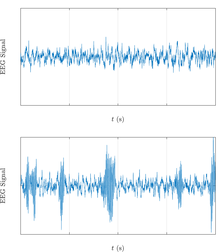
Figure 3: EEG time series at channel O2
As an illustration, we show the EEG time series at channels O2 and P4 in the
alert and fatigue states. There is clear intermittency in the O2 time series in the
fatigue state. This is depicted by a singularity at a frequency in the range 100 < ω <
300 in its periodogram. The appearance of this frequency for intermittency is likely
due to the closed eye tendency when a driver is tired. Similar strong intermittency
is found in the P4 time series in the fatigue state.
The spectral slopes of the O2 and P4 time series at low frequencies (ω ≤ 100)
are β = 1.33 and 1.23 respectively for the alert state, and β = 1.37 and 1.28
respectively for the fatigue state. These slopes are obtained via the regression of
log f (λ) against log |λ| based on the 1/f
β
-noise model log f (λ) ∼ −β log |λ| as λ →
0. The estimated slopes indicate that the alert-state time series are nonstationary
and possess short-range dependence with H = 0.165 and 0.115 respectively using
the formula 2H + 1 = β. The Hurst indices are H = 0.185 and 0.14 for O2 and P4
respectively in the fatigue state, indicating that there is no significant change (in
the low-frequency behaviour of these time series) from the alert state to the fatigue
state.
19
.CC-BY-NC-ND 4.0 International licensemade available under a
(which was not certified by peer review) is the author/funder, who has granted bioRxiv a license to display the preprint in perpetuity. It is
The copyright holder for this preprintthis version posted August 4, 2020. ; https://doi.org/10.1101/2020.08.03.234120doi: bioRxiv preprint

10
2
10
-6
10
-4
10
-2
10
0
Alert state, Channel O2
10
2
10
-6
10
-4
10
-2
10
0
Fatigue state, Channel O2
Figure 4: Log-periodogram of the EEG time series at channel O2 shown in Fig. 3
5.3.2. Global power-law scaling
The covariance function of (2.15) is of the form
R(t) = |t|
−κ
L(t), t ∈ R, (5.1)
with 0 < κ < 1 for 1 < α < 2, and L (x) being a function slowly varying at infinity.
A Tauberian theorem [27, p. 66] implies that the spectral density f(λ) corresponding
to R(t) behaves as
f(λ) ∼ c(κ)L
1
|λ|
|λ|
κ−1
(5.2)
as |λ| → 0, where the Tauberian constant c(κ) =
Γ
(
1−κ
2
)
2
κ
√
πΓ(κ/2)
. Thus, at a fixed loca-
tion, the asymptotic solution of (2.12) behaves as 1/f
β
-noise, with β = 2 (1 − 1/α).
Consequently, the parameter α of the fractional diffusion operator (−∆
S
2
)
α/2
(I − ∆
S
2
)
γ/2
of (1.1) quantifies its 1/f
2
(
1−
1
α
)
-noise behaviour at low frequencies. Under the as-
sumptions of this global model, there may not be any formula connecting this low-
frequency behaviour via β = 2 (1 − 1/α) with the bahaviour via β = 2H + 1 of
the EEG time series investigated above because the α-component in the operator
(−∆
S
2
)
α/2
(I − ∆
S
2
)
γ/2
picks up only a part of the memory in the EEG global field.
The remaining part is embedded in the delay operator (−∆
S
2
)
1/2
u(t − τ, x). How-
ever, as described, this 1/f
2
(
1−
1
α
)
-noise behaviour can be used as an indicator to
distinguish between the alert and fatigue states. This interpretation is included in
the next subsection.
5.3.3. Behaviour of global EEG
We use (4.7) and (4.13) to estimate the parameters α, γ and the delay parameter
τ as well as the exponent θ. In the optimization problem (4.8), we set L
1
= 30
and L
2
= 50. Table 1 reports the numerical estimates and standard deviations of
α, α + γ, τ and θ averaged over a sample of up to 50 participants in the alert and
fatigue states. For each participant, we use EEG measurements over 20 seconds at
all 32 channels on the scalp. Fig. 7 plots the paths of the estimated values of α, α+γ
and τ over these participants.
First of all, the averaged value α = 1.116 in Table 1 for the fatigue state yields
β = 0.21, hence κ = 0.79 in the spectral density (5.2). This result indicates that
global EEG exhibits long memory, hence global power-law scaling in the fatigue
20
.CC-BY-NC-ND 4.0 International licensemade available under a
(which was not certified by peer review) is the author/funder, who has granted bioRxiv a license to display the preprint in perpetuity. It is
The copyright holder for this preprintthis version posted August 4, 2020. ; https://doi.org/10.1101/2020.08.03.234120doi: bioRxiv preprint

0 5 10 15 20
-50
0
50
EEG signal, Alert state, Channel P4
0 5 10 15 20
-50
0
50
EEG signal, Fatigue state, Channel P4
Figure 5: EEG time series at channel P4
state, as predicted by the covariance function (5.1) and the spectral density (5.2).
The path of α in Fig. 7 also shows that α is consistently larger than 1 over the
sample of participants, hence exhibiting power-law scaling in the fatigue state. The
averaged value of α smaller but close to 1 for the alert state in Table 1 does not
lend support for the assertion of long memory in the alert state. This would indi-
cate weakly dependent non-stationarity rather than strongly dependent stationarity
in the solution for the alert state. This agrees with the assertion of higher non-
Gaussianity in the alert state, which we discuss next.
The estimates of α and α + γ are obtained for t sufficiently large. The value of α
around 1 in Table 1 confirms that global EEG is α-stable in both alert and fatigue
states. This degree of non-Gaussianity is distinct from the Gaussianity of standard
diffusion when α = 2. It demonstrates the fractal effect due to a multifractal medium
on the diffusion as anticipated in Eq. (2.11). The result agrees with the diffusion
of EEG signals through a heterogeneous medium due to the flow of current in a
conductive fluid and the high density of membranes as heralded in [7]. The lower
value of α in Table 1 and consistently over the entire sample of participants in Fig. 7
21
.CC-BY-NC-ND 4.0 International licensemade available under a
(which was not certified by peer review) is the author/funder, who has granted bioRxiv a license to display the preprint in perpetuity. It is
The copyright holder for this preprintthis version posted August 4, 2020. ; https://doi.org/10.1101/2020.08.03.234120doi: bioRxiv preprint

10
2
10
-6
10
-4
10
-2
10
0
Alert state, Channel P4
Alert state
10
2
10
-6
10
-4
10
-2
10
0
Fatigue state, Channel P4
Fatigue state
Figure 6: Log-periodogram of the EEG time series at channel P4 shown in Fig. 5
for the alert state indicates that global EEG has larger jumps and more rugged paths
in the alert state than in the fatigue state. The lower value of α + γ, in Table 1 and
Fig. 7, corroborates the assertion that paths of global EEG are more multifractal in
the alert state than in the fatigue state. All these interpretations are suggested by
the analytical results of the fractional diffusion model of Subsection 2.3.
The mean value of the delay parameter τ in Table 1 is obtained under the
assumption that the delay response is due to the initial condition, that is, when the
alert or fatigue state starts. Hence τ is evaluated as t → 0 in the estimation scheme.
The larger value of τ shown in Table 1 indicates that global EEG has longer delay,
hence stronger memory, in the alert state than in the fatigue state. This result is
also maintained consistently over the sample of participants in Fig. 7.
The above analysis confirms the occurrence of strong response of the system
to the initial state within the context of non-Gaussian diffusion. The occurence is
intuitively consistent with the behaviour of a driver in the alert or fatigue state.
The results provide additional tools to construct global indicators to distinguish
between these two states of brain activity complementing those afforded by time-
series techniques.
Table 1: Averages and standard deviations of the parameters α, α + γ, τ and θ over up
to 50 participants
Average α α + γ τ θ
Alert 0.921 ± 0.207 1.676 ± 0.141 0.183 ± 0.061 2.323 ± 0.042
Fatigue 1.116 ± 0.208 1.773 ± 0.132 0.160 ± 0.048 2.334 ± 0.041
Acknowledgements
Hung T. Nguyen acknowledges support from the Australian Research Council
under Discovery Project DP150102493. Yu Guang Wang acknowledges the support
of funding from the European Research Council (ERC) under the European Union’s
Horizon 2020 research and innovation programme (grant agreement n
o
757983).
22
.CC-BY-NC-ND 4.0 International licensemade available under a
(which was not certified by peer review) is the author/funder, who has granted bioRxiv a license to display the preprint in perpetuity. It is
The copyright holder for this preprintthis version posted August 4, 2020. ; https://doi.org/10.1101/2020.08.03.234120doi: bioRxiv preprint

(a) α (b) α + γ (c) τ
Figure 7: Paths of fractional diffusion exponents α, α + γ and delay parameter τ over a
sample of up to 50 participants
References
[1] T.
˚
Akerstedt, G. Kecklund, and A. Knutsson, Manifest sleepiness and
the spectral content of the EEG during shift work, Sleep, 14 (1991), pp. 221–225.
[2] J. Angulo, M. Ruiz-Medina, V. Anh, and W. Grecksch, Fractional dif-
fusion and fractional heat equation, Advances in Applied Probability, 32 (2000),
pp. 1077–1099.
[3] V. Anh, J. Angulo, and M. Ruiz-Medina, Possible long-range dependence
in fractional random fields, Journal of Statistical Planning and Inference, 80
(1999), pp. 95–110.
[4] V. Anh and C. Nguyen, Stochastic analysis of fractional riesz-bessel motion,
Random Operators and Stochastic Equations, 8 (2000), pp. 105–126.
[5] V. V. Anh and R. McVinish, The Riesz-Bessel fractional diffusion equation,
Applied Mathematics and Optimization, 49 (2004), pp. 241–264.
[6] P. Bak, How nature works: the science of self-organized criticality, Springer
Science & Business Media, 2013.
[7] C. B
´
edard and A. Destexhe, Macroscopic models of local field potentials
and the apparent 1/f noise in brain activity, Biophysical Journal, 96 (2009),
pp. 2589–2603.
[8] C. B
´
edard, H. Kroeger, and A. Destexhe, Does the 1/f frequency scaling
of brain signals reflect self-organized critical states?, Physical Review Letters,
97 (2006), p. 118102.
[9] J. M. Beggs and N. Timme, Being critical of criticality in the brain, Frontiers
in Physiology, 3 (2012).
[10] G. Buzsaki, C. A. Anastassiou, and C. Koch, The origin of extracellular
fields and currents - EEG, ECoG, LFP and spikes, Nature Reviews Neuro-
science, 13 (2012), pp. 407–420.
[11] J. Connor, R. Norton, S. Ameratunga, E. Robinson, I. Civil,
R. Dunn, J. Bailey, and R. Jackson, Driver sleepiness and risk of se-
rious injury to car occupants: population based case control study, BMJ, 324
(2002), p. 1125.
23
.CC-BY-NC-ND 4.0 International licensemade available under a
(which was not certified by peer review) is the author/funder, who has granted bioRxiv a license to display the preprint in perpetuity. It is
The copyright holder for this preprintthis version posted August 4, 2020. ; https://doi.org/10.1101/2020.08.03.234120doi: bioRxiv preprint
[12] A. Craig, Y. Tran, N. Wijesuriya, and H. Nguyen, Regional brain wave
activity changes associated with fatigue, Psychophysiology, 49 (2012), pp. 574–
582.
[13] F. Dai and Y. Xu, Approximation theory and harmonic analysis on spheres
and balls, Springer Monographs in Mathematics, Springer, New York, 2013.
[14] R. Dautray and J.-L. Lions, Mathematical Analysis and Numerical Meth-
ods for Science and Technology. Vol. 3. Spectral Theory and Applications,
Springer-Verlag, Berlin, 1990.
[15] M. C. Delfour and S. K. Mitter, Hereditary differential systems with
constant delays. i. general case, Journal of Differential Equations, 12 (1972),
pp. 213–235.
[16] S. El Boustani, O. Marre, S. B
´
ehuret, P. Baudot, P. Yger, T. Bal,
A. Destexhe, and Y. Fr
´
egnac, Network-state modulation of power-law
frequency-scaling in visual cortical neurons, PLoS Computational Biology, 5
(2009), p. e1000519.
[17] T. Faria, Normal forms and hopf bifurcation for partial differential equations
with delays, Transactions of the American Mathematical Society, 352 (2000),
pp. 2217–2238.
[18] D. P. Francis, K. Willson, L. C. Davies, A. J. Coats, and
M. Piepoli, Quantitative general theory for periodic breathing in chronic heart
failure and its clinical implications, Circulation, 102 (2000), pp. 2214–2221.
[19] W. Freeden and M. Schreiner, Spherical functions of mathematical geo-
sciences: a scalar, vectorial, and tensorial setup, Springer Science & Business
Media, 2008.
[20] B. J. He, Scale-free properties of the functional magnetic resonance imaging
signal during rest and task, Journal of Neuroscience, 31 (2011), pp. 13786–
13795.
[21] K. Hesse and R. S. Womersley, Numerical integration with polynomial
exactness over a spherical cap, Advances in Computational Mathematics, 36
(2012), pp. 451–483.
[22] Y. Hu and D. Nualart, Parameter estimation for fractional ornstein–
uhlenbeck processes, Statistics & Probability Letters, 80 (2010), pp. 1030–1038.
[23] H. J. Jensen, Self-organized criticality: emergent complex behavior in physical
and biological systems, vol. 10, Cambridge university press, 1998.
[24] T. Kato, Perturbation theory for linear operators, Springer-Verlag New York,
Inc., New York, 1966.
[25] J. Keiner, S. Kunis, and D. Potts, Using NFFT 3—a software library for
various nonequispaced fast fourier transforms, ACM Transactions on Mathe-
matical Software (TOMS), 36 (2009), p. 19.
24
.CC-BY-NC-ND 4.0 International licensemade available under a
(which was not certified by peer review) is the author/funder, who has granted bioRxiv a license to display the preprint in perpetuity. It is
The copyright holder for this preprintthis version posted August 4, 2020. ; https://doi.org/10.1101/2020.08.03.234120doi: bioRxiv preprint

[26] S. Kunis and D. Potts, Fast spherical fourier algorithms, Journal of Com-
putational and Applied Mathematics, 161 (2003), pp. 75–98.
[27] N. Leonenko, Limit theorems for random fields with singular spectrum,
vol. 465, Springer Science & Business Media, 1999.
[28] C. M
¨
uller, Spherical Harmonics, Springer-Verlag, Berlin-New York, 1966.
[29] S. D. Muthukumaraswamy and D. T. Liley, 1/f electrophysiological spec-
tra in resting and drug-induced states can be explained by the dynamics of mul-
tiple oscillatory relaxation processes, NeuroImage, 179 (2018), pp. 582–595.
[30] S.-i. Nakagiri, On the fundamental solution of delay-differential equations in
Banach spaces, Journal of Differential Equations, 41 (1981), pp. 349–368.
[31] B. Øksendal, Stochastic differential equations. An introduction with applica-
tions, Universitext, Springer-Verlag, Berlin, sixth ed., 2003.
[32] M. D. Ruiz-Medina, V. V. Anh, and J. M. Angulo, Multifractional
Markov processes in heterogeneous domains, Stochastic Analysis and Applica-
tions, 29 (2011), pp. 15–47.
[33] O. R. Ryynanen, J. A. Hyttinen, and J. A. Malmivuo, Effect of mea-
surement noise and electrode density on the spatial resolution of cortical poten-
tial distribution with different resistivity values for the skull, IEEE Transactions
on Biomedical Engineering, 53 (2006), pp. 1851–1858.
[34] E. M. Stein, Singular integrals and differentiability properties of functions,
Princeton University Press, Princeton, N.J., 1970.
[35] Y. G. Wang and X. Zhuang, Tight framelets and fast framelet filter bank
transforms on manifolds, Applied and Computational Harmonic Analysis, 48
(2020), pp. 64–95.
Appendix A. Fundamental solution of delay-differential equations
In order to derive the solution of the system (1.1) and (1.2), we recall the following
theory of fundamental solution of delay-differential equations in Banach spaces due
to [30]. Let E be a Banach space. We denote by B(E) the Banach space of all
bounded linear operators from E into itself. We consider the following differential
system with m delay terms:
du(t)
dt
= Au(t) +
m
X
r=1
A
r
u(t − rτ) + f(t), t ≥ 0, (A.1)
u(0) = u
0
, u(s) = g(s), s ∈ [−mτ, 0), (A.2)
where τ > 0 is a constant, u(t), f(t), g(t) ∈ E. The operators A and A
r
, r = 1, ..., m,
possibly unbounded, are assumed to satisfy the following assumptions:
H
0
. The operator A generates a strongly continuous semigroup {T (t), t ≥ 0} on
E;
25
.CC-BY-NC-ND 4.0 International licensemade available under a
(which was not certified by peer review) is the author/funder, who has granted bioRxiv a license to display the preprint in perpetuity. It is
The copyright holder for this preprintthis version posted August 4, 2020. ; https://doi.org/10.1101/2020.08.03.234120doi: bioRxiv preprint
H
1
. The A
r
, r = 1, ..., m, are closed linear operators with dense domains D(A
r
) in
E;
H
q
2
. For each r, there exists a function M
r
(·) ∈ L
q
([0, τ]) such that kT (t)A
r
uk ≤
M
r
(t)kuk for almost all t ∈ [0, τ] and all u ∈ D(A
r
).
Let u
0
∈ E, f ∈ L
loc
p
(R
+
; E) , g ∈ L
p
0
(−mτ, 0; E) be given, and let Assumption
H
q
0
2
with 1/p
0
+ 1/q
0
= 1 be satisfied, where p, p
0
∈ [1, ∞]. Then, the function
u(t; u
0
, f, g) = T (t)u
0
+
Z
t
0
T (t −s)f(s)ds +
m
X
r=1
Z
t
0
(T (t −s)A
r
)g(s −rτ)ds (A.3)
is well defined and is strongly continuous on [0, τ ]. This function is defined to be
the mild solution of the system (A.1) and (A.2), see [30].
Let now f = 0, g = 0 and let Assumptions H
0
, H
1
and H
1
2
be satisfied. Then,
as given by (A.3), the mild solution u(t; u
0
) = u(t; u
0
, 0, 0) can be constructed for
any u
0
∈ E. The mapping G : R
+
× E → E defined by G(t, u
0
) = u(t; u
0
) generates
a one-parameter family of bounded operators {G(t), t ≥ 0}, where G(t) is defined
by G(t)u = G(t, u) for u ∈ E and satisfies
(i) G(t) = T (t) for all t ∈ [0, τ] and G(t) ∈ B(E) for all t ≥ 0;
(ii) for each u
0
∈ E, G(t)u
0
is continuous on R
+
.
By [30], we can define the function G(t) as the fundamental solution of Eq. (A.1).
From the given semigroup {T (t), t ≥ 0} we define the operators T
1
(t), . . . , T
k
(t),
t ≥ 0, inductively by
T
1
(t) = T (t)
T
k
(t) =
min(k−1,m)
X
i=1
Z
t
0
T (t − s)A
i
T
k−1
(s)ds for k = 2, 3, . . . (A.4)
From (A.4), an explicit form of T
k
(t) can be derived. We first define the index sets
Λ(j, k) for all j, k = 1, 2, . . . by
Λ(j, k) = {(i
1
, . . . , i
j
) : 1 ≤ i
1
, . . . , i
j
≤ m and i
1
+ ··· + i
j
= k}.
Note that Λ(j, k) = ∅ for j > k. The following integral expression of T
k
(t) for k ≥ 2
is then obtained:
T
k
(t) =
k−1
X
j=1
X
Λ(j,k−1)
Z
t
0
T (t −s
j−1
)A
i
1
···
Z
s
1
0
T (s
1
−s)A
i
j
T (s)dsds
1
. . . ds
j−1
. (A.5)
Summarising, we obtain the following result, which is given by [30, Theorem 3.1].
Theorem Appendix A.1. Let Assumptions H
0
, H
1
and H
1
2
be satisfied. Then the
set of one-parameter family of strongly continuous operators {T
k
(·) : k = 1, 2, ...}
can be constructed as in (A.5), and the fundamental solution G(t), t ≥ 0, is given
by
G(t) =
k
X
i=1
T
i
(t − (i − 1)τ),
where t ∈ [(k − 1)τ, kτ ].
26
.CC-BY-NC-ND 4.0 International licensemade available under a
(which was not certified by peer review) is the author/funder, who has granted bioRxiv a license to display the preprint in perpetuity. It is
The copyright holder for this preprintthis version posted August 4, 2020. ; https://doi.org/10.1101/2020.08.03.234120doi: bioRxiv preprint

We introduce an additional condition:
H
3
. For each r, A
r
commutes with T (t) for all t ≥ 0, i.e., for any u ∈ D(A
r
) and
t ≥ 0, T (t)u ∈ D(A
r
) and A
r
T (t)u = T (t)A
r
u.
Then, by H
3
and (A.5), T
k
(t) is given formally by
T
k
(t) =
k−1
X
j=1
X
Λ(j,k−1)
t
j
j!
T (t)A
i
1
. . . A
i
j
, k = 2, 3, ...
Consequently, G(t), t ∈ [(k − 1) τ, kτ], is represented formally as
G(t) = T (t) +
k
X
i=2
i−1
X
j=1
X
Λ(j,i−1)
1
j!
(t − (i − 1)τ)
j
T (t − (i − 1)τ)A
i
1
. . . A
i
j
. (A.6)
The mild solution (A.3) can then be given in terms of G(t) as
u(t; u
0
, f, g) = G(t)u
0
+
Z
t
0
G(t−s)f(s)ds+
m
X
r=1
Z
0
−rτ
G(t−rτ −s)A
r
g(s)ds, (A.7)
where G(s)A
r
= O, the null operator on E, if s < 0. This is given by [30, Theo-
rem 4.2].
27
.CC-BY-NC-ND 4.0 International licensemade available under a
(which was not certified by peer review) is the author/funder, who has granted bioRxiv a license to display the preprint in perpetuity. It is
The copyright holder for this preprintthis version posted August 4, 2020. ; https://doi.org/10.1101/2020.08.03.234120doi: bioRxiv preprint
