
PhD Dissertation
Continuous-Time Modeling Using
Lévy-Driven Moving Averages
Representations, Limit Theorems and Other Properties
Mikkel Slot Nielsen
Department of Mathematics
Aarhus University
2019
Continuous-time modeling using Lévy-driven moving averages
Representations, limit theorems and other properties
PhD dissertation by
Mikkel Slot Nielsen
Department of Mathematics, Aarhus University
Ny Munkegade 118, 8000 Aarhus C, Denmark
Supervised by
Associate Professor Andreas Basse-O’Connor
Associate Professor Jan Pedersen
Submitted to Graduate School of Science and Technology, Aarhus, July 3, 2019
Dissertation was typesat in kpfonts with
pdfL
A
T
E
X and the memoir class
DEPARTMENT OF MATHEMATICS
AARHUS
UNIVERSITY
AU
Contents
Preface . . . . . . . . . . . . . . . . . . . . . . . . . . . . . . . . . . . . . . . . . v
Summary . . . . . . . . . . . . . . . . . . . . . . . . . . . . . . . . . . . . . . . . vii
Resumé . . . . . . . . . . . . . . . . . . . . . . . . . . . . . . . . . . . . . . . . . ix
Introduction 1
1 A Wold–Karhunen type decomposition and the Lévy-driven
moving averages . . . . . . . . . . . . . . . . . . . . . . . . . . . 1
2 Dynamic models for Lévy-driven moving averages . . . . . . . 6
3
Limit theorems for quadratic forms and related quantities of
Lévy-driven moving averages . . . . . . . . . . . . . . . . . . . 16
References . . . . . . . . . . . . . . . . . . . . . . . . . . . . . . . . . 19
Paper A Equivalent martingale measures for Lévy-driven moving
averages and related processes 23
by Andreas Basse-O’Connor, Mikkel Slot Nielsen and Jan Pedersen
1 Introduction and a main result . . . . . . . . . . . . . . . . . . . 23
2 Further main results . . . . . . . . . . . . . . . . . . . . . . . . . 26
3 Preliminaries . . . . . . . . . . . . . . . . . . . . . . . . . . . . . 30
4 Proofs . . . . . . . . . . . . . . . . . . . . . . . . . . . . . . . . . 31
References . . . . . . . . . . . . . . . . . . . . . . . . . . . . . . . . . 41
Paper B Stochastic delay differential equations and related
autoregressive models 45
by Andreas Basse-O’Connor, Mikkel Slot Nielsen, Jan Pedersen
and Victor Rohde
1 Introduction . . . . . . . . . . . . . . . . . . . . . . . . . . . . . 45
2 The SDDE setup . . . . . . . . . . . . . . . . . . . . . . . . . . . 48
3 The level model . . . . . . . . . . . . . . . . . . . . . . . . . . . 54
4 Proofs and technical results . . . . . . . . . . . . . . . . . . . . 58
References . . . . . . . . . . . . . . . . . . . . . . . . . . . . . . . . . 65
Paper C Recovering the background noise of a Lévy-driven CARMA
process using an SDDE approach 69
by Mikkel Slot Nielsen and Victor Rohde
1 Introduction . . . . . . . . . . . . . . . . . . . . . . . . . . . . . 69
2 CARMA processes and their dynamic SDDE representation . . 70
i
3 Estimation of the SDDE parameters . . . . . . . . . . . . . . . . 74
4 A simulation study, p = 2 . . . . . . . . . . . . . . . . . . . . . . 75
5 Conclusion and further research . . . . . . . . . . . . . . . . . . 77
References . . . . . . . . . . . . . . . . . . . . . . . . . . . . . . . . . 78
Paper D Multivariate stochastic delay differential equations and CAR
representations of CARMA processes 81
by Andreas Basse-O’Connor, Mikkel Slot Nielsen, Jan Pedersen and
Victor Rohde
1 Introduction and main ideas . . . . . . . . . . . . . . . . . . . . 81
2 Notation . . . . . . . . . . . . . . . . . . . . . . . . . . . . . . . 83
3 Stochastic delay differential equations . . . . . . . . . . . . . . 85
4 Examples and further results . . . . . . . . . . . . . . . . . . . . 86
5 Proofs and auxiliary results . . . . . . . . . . . . . . . . . . . . 93
References . . . . . . . . . . . . . . . . . . . . . . . . . . . . . . . . . 105
Paper E Stochastic differential equations with a fractionally filtered delay:
a semimartingale model for long-range dependent processes 107
by Richard A. Davis, Mikkel Slot Nielsen and Victor Rohde
1 Introduction . . . . . . . . . . . . . . . . . . . . . . . . . . . . . 107
2 Preliminaries . . . . . . . . . . . . . . . . . . . . . . . . . . . . . 111
3 The stochastic fractional delay differential equation . . . . . . . 112
4 Delays of exponential type . . . . . . . . . . . . . . . . . . . . . 116
5 Simulation from the SFDDE . . . . . . . . . . . . . . . . . . . . 120
6 Proofs . . . . . . . . . . . . . . . . . . . . . . . . . . . . . . . . . 123
7 Supplement . . . . . . . . . . . . . . . . . . . . . . . . . . . . . 131
References . . . . . . . . . . . . . . . . . . . . . . . . . . . . . . . . . 134
Paper F Limit theorems for quadratic forms and related quantities of
discretely sampled continuous-time moving averages 137
by Mikkel Slot Nielsen and Jan Pedersen
1 Introduction . . . . . . . . . . . . . . . . . . . . . . . . . . . . . 137
2 Preliminaries . . . . . . . . . . . . . . . . . . . . . . . . . . . . . 141
3 Further results and examples . . . . . . . . . . . . . . . . . . . 142
4 Proofs . . . . . . . . . . . . . . . . . . . . . . . . . . . . . . . . . 147
References . . . . . . . . . . . . . . . . . . . . . . . . . . . . . . . . . 156
Paper G On non-stationary solutions to MSDDEs: representations and
the cointegration space 159
by Mikkel Slot Nielsen
1 Introduction and main results . . . . . . . . . . . . . . . . . . . 159
2 Preliminaries . . . . . . . . . . . . . . . . . . . . . . . . . . . . . 162
3
General results on existence, uniqueness and representations
of solutions to MSDDEs . . . . . . . . . . . . . . . . . . . . . . . 163
ii
4 Cointegrated multivariate CARMA processes . . . . . . . . . . 168
5 Proofs . . . . . . . . . . . . . . . . . . . . . . . . . . . . . . . . . 170
References . . . . . . . . . . . . . . . . . . . . . . . . . . . . . . . . . 179
Paper H Low frequency estimation of Lévy-driven moving averages 181
by Mikkel Slot Nielsen
1 Introduction . . . . . . . . . . . . . . . . . . . . . . . . . . . . . 181
2 Estimators of interest and asymptotic results . . . . . . . . . . 183
3 Examples . . . . . . . . . . . . . . . . . . . . . . . . . . . . . . . 186
References . . . . . . . . . . . . . . . . . . . . . . . . . . . . . . . . . 190
Paper I A statistical view on a surrogate model for estimating extreme
events with an application to wind turbines 193
by Mikkel Slot Nielsen and Victor Rohde
1 Introduction . . . . . . . . . . . . . . . . . . . . . . . . . . . . . 193
2 The model . . . . . . . . . . . . . . . . . . . . . . . . . . . . . . 195
3 Application to extreme event estimation for wind turbines . . . 198
4 Conclusion . . . . . . . . . . . . . . . . . . . . . . . . . . . . . . 204
References . . . . . . . . . . . . . . . . . . . . . . . . . . . . . . . . . 205
iii
Preface
This dissertation is the result of my PhD studies carried out from May 1, 2015 to
July 3, 2019 at Department of Mathematics, Aarhus University, under supervision
of Andreas Basse-O’Connor (main supervisor) and Jan Pedersen (co-supervisor). My
studies were fully funded by Andreas’ grant (DFF–4002–00003) from the Danish
Council for Independent Research.
The dissertation consists of the following nine self-contained papers:
Paper A
Equivalent martingale measures for Lévy-driven moving averages and
related processes. Stochastic Processes and their Applications 128(8), 2538–
2556.
Paper B
Stochastic delay differential equations and related autoregressive models.
Stochastics (forthcoming), 24 pages.
Paper C
Recovering the background noise of a Lévy-driven CARMA process using
an SDDE approach. Proceedings ITISE 2017 2, 707–718.
Paper D
Multivariate stochastic delay differential equations and CAR representa-
tions of CARMA processes. Stochastic Processes and their Applications (forth-
coming), 25 pages.
Paper E
Stochastic differential equations with a fractionally filtered delay: a semi-
martingale model for long-range dependent processes. Bernoulli (forthcom-
ing), 30 pages.
Paper F
Limit theorems for quadratic forms and related quantities of discretely
sampled continuous-time moving averages. ESAIM: Probability and Statistics
(forthcoming), 20 pages.
Paper G
On non-stationary solutions to MSDDEs: representations and the cointe-
gration space. Submitted.
Paper H Low frequency estimation of Lévy-driven moving averages. Submitted.
Paper I
A statistical view on a surrogate model for estimating extreme events with
an application to wind turbines. In preparation.
Up to notation and minor adjustments, Papers A–H align with their published or
submitted version. Main parts of Papers A–C are written during the first two years of
my PhD studies, and thus these were also included in my progress report used for
the qualifying examination, after which I obtained a master’s degree in mathematical
economics. While a few of the ideas of Papers D and F were briefly discussed in the
v
Preface
progress report as well, Papers D–I are primarily a result of the last two years of
my studies. I have contributed comprehensively in both the writing as well as the
research phase of Papers A–B and D–H. Together with Victor Rohde I have written
Papers C and I, and to these we have contributed equally.
The first chapter of the dissertation is an introduction, which motivates the use of
Lévy-driven moving averages in the modeling of continuous-time stochastic systems
and discusses the importance of obtaining knowledge of their representations, limit
theorems and certain other properties. The findings of Papers A–H deliver answers
to many of the questions raised in this discussion, and hence the main results of
these papers will also be highlighted in this chapter. Paper I, however, is an industrial
collaboration with Vestas Wind Systems A/S and concerns estimation of extreme
loads on wind turbines using covariates. Since the details are carefully explained in
the included paper and the overall aim differs from that of Papers A–H, I have chosen
not to address its findings in the introductory chapter.
My four years of PhD studies have been both challenging and rewarding, and I
owe several people huge thanks for making the journey joyful. First of all, I thank my
main supervisor Andreas Basse-O’Connor for giving me the unique opportunity of
pursuing a PhD degree in a truly inspiring and intellectually stimulating research
environment and for our many fruitful discussions. His support, enthusiasm and
high ambitions have definitely pushed my limits as a researcher. A special thanks
goes to my co-supervisor Jan Pedersen, with whom I have had uncountably many
conversations spanning from technical details in proofs and general probabilistic
and statistical considerations to an analysis of the outcome of yesterday’s hockey
match. Due to his extraordinary guidance, his trust in my abilities and his positive
mindset, Jan has had a significant impact on my development and well-being during
my studies. I feel honored that Andreas and Jan have invested this much time and
effort in me—it exceeds by far what could be expected of a supervisor, and for this I
am deeply grateful.
I would also like to thank my co-author Richard A. Davis from Department of
Statistics, Columbia University, for letting me visit him and his group in New York and
for his interest in my research. Our frequent meetings and his generous hospitality
ensured that I had a constructive and pleasant stay. I thank as well my office mate
Victor Rohde for numerous fruitful collaborations, and the local L
A
T
E
X expert Lars
‘daleif’ Madsen and my office mate Mathias Ljungdahl for helping me with the
technical typesetting. Furthermore, I want to thank my colleagues at Department
of Mathematics, Aarhus University, for giving me a perfect working environment,
which I have enjoyed being a part of throughout my studies. A particular thanks goes
to Claudio Heinrich, Julie Thøgersen, Mads Stehr, Mathias Ljungdahl, Patrick Laub,
Thorbjørn Grønbæk and Victor Rohde for all the (non-)mathematical discussions and
social activities.
Finally, my family and friends deserve an abundance of gratitude for their endless
support and encouragement. I conclude with a very special thanks to my fiancée
Marianne, since none of this would have been possible without her.
Mikkel Slot Nielsen
Aarhus, July 2019
vi
Summary
Similarly to the discrete-time framework, moving averages driven by white noise
processes play a crucial role in the modeling of continuous-time stochastic processes.
The main purpose of this dissertation is to address various aspects of Lévy-driven
moving averages. The existence of equivalent martingale measures, autoregressive
representations and limit theorems will be of particular interest.
Based on earlier literature on the semimartingale property for Lévy-driven moving
averages, and under rather general conditions on the Lévy process, we give necessary
and sufficient conditions on the driving kernel for an equivalent martingale measure
to exist. In particular, these conditions extend previous results for Gaussian moving
averages to the symmetric α-stable case with an arbitrary α ∈ (1, 2].
A significant part of the dissertation concerns various properties of solutions to
a range of stochastic delay differential equations (SDDEs). Among other things, we
obtain sufficient conditions for existence and uniqueness of solutions to univariate,
multivariate, higher order and fractional SDDEs, provide moving average represen-
tations of the solutions and discuss its memory properties. A few implications of
the obtained results are that (i) invertible continuous-time ARMA processes can
be viewed as unique solutions to SDDEs, (ii) solutions can be semimartingales and
exhibit long memory at the same time, and (iii) cointegration can be embedded in
multivariate SDDEs in a straightforward manner. From the properties that we prove
for SDDEs we draw several parallels to classical results for autoregressive representa-
tions in the discrete-time literature and, hence, indicate that it may be reasonable to
think of SDDEs as the continuous-time counterpart.
We also study the limiting behavior of quadratic forms and related quantities of
discretely sampled Lévy-driven moving averages. The linear nature of Lévy-driven
moving averages and their tractable probabilistic structure allow us to obtain rather
explicit conditions on the driving kernel and the coefficients of the quadratic form
ensuring asymptotic normality. The result differs from those obtained in related
literature due to the quite delicate interplay between discrete-time sampling and
continuous-time convolutions. The applications of these asymptotic results are many;
in particular, we demonstrate how they can be used to obtain central limit theorems
when estimating the driving kernel parametrically using least squares.
The last part of the dissertation is related to an industrial collaboration, where
we consider prediction of extreme loads on wind turbines using only a number of
covariates and a simulation tool. In particular, we discuss how to set up a statistical
model in this situation, address some of the key assumptions and, finally, check its
performance on real-world data.
vii
Resumé
Præcis som for modeller i diskret tid spiller glidende gennemsnit drevet af hvid støj
en fundamental rolle i modelleringen af stokastiske processer i kontinuert tid. Hoved-
formålet med denne afhandling er at undersøge forskellige aspekter af Lévy-drevne
glidende gennemsnit. Vi vil være særligt interesserede i eksistens af ækvivalente
martingalmål, autoregressive repræsentationer og grænseværdisætninger.
Baseret på tidligere litteratur om semimartingal-egenskaben for Lévy-drevne
glidende gennemsnit, og under ret svage antagelser på Lévy-processen, giver vi nød-
vendige og tilstrækkelige betingelser på den drivende kerne, der sikrer, at et ækvi-
valent martingalmål eksisterer. Som et specialtilfælde af dette resultat opnår vi en
generalisering af resultater for gaussiske glidende gennemsnit til det symmetrisk
α-stabile tilfælde for et vilkårligt α ∈ (1,2].
En stor del af afhandlingen omhandler forskellige egenskaber ved løsninger til en
række stokastiske differentialligninger, som involverer processens egen fortid (disse
vil herfra kort refereres til som SDDEer). Vi giver tilstrækkelige betingelser til at
sikre eksistens og entydighed af løsninger til en- og flerdimensionale SDDEer, SD-
DEer af højere orden og fraktionelle SDDEer. Desuden repræsenterer vi løsningerne
som glidende gennemsnit samt studerer deres afhængighedsstruktur. Umiddelbare
konsekvenser af disse resultater er, at (i) invertible ARMA processer i kontinuert tid
er entydige løsninger til SDDEer, (ii) løsninger kan være semimartingaler og have
lang hukommelse på samme tid, og (iii) kointegration kan nemt indlejres i de fler-
dimensionale SDDEer. Fra de beviste egenskaber for SDDEer trækker vi adskillige
paralleller til klassiske resultater for autoregressive modeller i diskret tid og indikerer
på den måde, at SDDEer kan opfattes som modstykket i kontinuert tid.
Vi studerer også den asymptotiske opførsel af kvadratiske former og relaterede
størrelser af diskrete observationer fra Lévy-drevne glidende gennemsnit. De gliden-
de gennemsnits lineære struktur samt transparente fordelingsmæssige egenskaber
gør det muligt for os at udlede eksplicitte betingelser på den drivende kerne og
koefficienterne i den kvadratiske form, som sikrer asymptotisk normalitet. På grund
af det udfordrende samspil mellem diskrete observationer og foldninger i kontinuert
tid adskiller resultatet sig fra dem, der er udledt i lignende litteratur. Sådanne asymp-
totiske resultater har mange anvendelser: f.eks. viser vi, hvordan de kan bruges til at
udlede centrale grænseværdisætninger ifm. parametrisk estimation af den drivende
kerne ved brug af mindste kvadraters metode.
Afhandlingens sidste del er relateret til et industrielt samarbejde, hvor vi studerer
estimation af ekstreme belastninger på vindmøller ved brug af en række kovariater
samt et simuleringsværktøj. Her diskuterer vi, hvordan man kan formulere en fornuf-
tig statistisk model samt belyser de væsentligste antagelser. Endeligt undersøger vi,
hvordan modellen klarer sig på data fra virkeligheden.
ix
Introduction
This chapter motivates the study of Lévy-driven moving average processes, highlights
key results obtained in the included papers and addresses their relation to existing
literature. In Section 1 we discuss why Lévy-driven moving averages constitute a
convenient class for modeling a wide range of stochastic systems in time by relying
on a Wold–Karhunen type decomposition, and we review some of their properties.
This leads naturally to a discussion of the key findings of Paper A. Section 2 concerns
the specification of the deterministic kernel driving the moving average. Specifically,
by drawing parallels to the discrete-time literature on ARMA type equations, we mo-
tivate the continuous-time ARMA processes as well as solutions to certain stochastic
delay differential equations. These are all special cases of moving averages, which
have formed the foundations of Papers B–E and G, and hence we end the section
by giving an overview of the main contributions of each of these papers. Finally, in
Section 3 we discuss the relevance of limit theorems for quadratic forms and related
quantities of Lévy-driven moving averages and relate it to Papers F and H.
1 A Wold–Karhunen type decomposition and the Lévy-driven
moving averages
There may be many reasons for modeling stochastic processes continuously in time.
To give an example, financial data are nowadays sampled at both very high and
irregular frequencies, and the continuous-time specification is a way to model this
type of observations in a consistent manner. Another reason is due to the remarkable
result of Delbaen and Schachermayer [18], which essentially characterizes arbitrage
opportunities in a financial market driven by semimartingales in terms of the exis-
tence of a so-called equivalent martingale measure (cf. Paper A). For further examples
on the use of continuous-time models, see [1, 8] and [22, Section 1.2].
Suppose now that (
X
t
)
t∈R
is a centered and weakly stationary (continuous-time)
process, that is,
E[X
2
t
] < ∞, E[X
t
] = 0 and
h 7−→E[X
t+h
X
t
]
=
h 7−→E[X
h
X
0
]
C γ
X
(1.1)
for all
t ∈ R
. While some phenomena may be reasonably described by such (
X
t
)
t∈R
,
one may often need to transform, deseasonalize and/or detrend observations to
align with such assumptions (see [11, Section 1.4] for details on this). A classical
example is the evolution of a stock price (
S
t
)
t∈R
exhibiting the random walk behavior
lim
t→∞
Var
(
S
t
) =
∞
, while its
∆
-period log-returns
X
t
=
logS
t+∆
−logS
t
,
t ∈ R
, might
approximately meet
(1.1)
. A related example is the (log-)prices of two stocks (
S
1
t
)
t∈R
and (
S
2
t
)
t∈R
, which individually may wander widely, but the spread
X
t
=
S
1
t
−S
2
t
,
t ∈ R
,
1

Introduction
behaves in a stationary manner. Such a situation can happen if the two stocks are
very similar by nature and one would in this case refer to them as being cointegrated
(see also Paper G). Despite the fact that the class of processes satisfying
(1.1)
is large
and general, Theorem 1.1 shows that these conditions are not far from ensuring that,
up to a term that can be perfectly predicted from the remote past (in an
L
2
(
P
) sense),
they correspond to moving averages driven by white noise processes. In the result it
will be required that (
X
t
)
t∈R
is continuous in
L
2
(
P
) or, equivalently,
γ
X
is continuous
at 0. Under this assumption it follows by Bochner’s theorem that there exists a finite
and symmetric Borel measure
F
X
, usually referred to as the spectral distribution of
(X
t
)
t∈R
, which has characteristic function γ
X
:
γ
X
(h) =
Z
R
e
ihy
F
X
(dy), h ∈ R. (1.2)
In the formulation,
f
X
refers to the density of the absolutely continuous part of
F
X
and sp denotes the L
2
(P) closure of the linear span.
Theorem 1.1 (Karhunen [28]).
Suppose that (
X
t
)
t∈R
is a centered and weakly station-
ary process, which is continuous in
L
2
(
P
). Moreover, suppose that the Paley–Wiener
condition
Z
R
|logf
X
(y)|
1 + y
2
dy < ∞ (1.3)
is satisfied. Then there exists a unique decomposition of (X
t
)
t∈R
as
X
t
=
Z
t
−∞
g(t −u) dZ
u
+ V
t
, t ∈ R, (1.4)
where
g : R → R
belongs to
L
2
, (
Z
t
)
t∈R
is a process with weakly stationary and orthogonal
increments satisfying
E
[(
Z
t
−Z
s
)
2
] =
t −s
for all
s < t
, and (
V
t
)
t∈R
is a weakly stationary
process with
V
t
∈
T
s∈R
sp{X
u
:
u ≤ s}
for
t ∈ R
. Moreover, if
F
X
is absolutely continuous
with a density f
X
satisfying (1.3) then V
t
= 0 for all t ∈ R.
The stochastic integral in
(1.4)
is defined as an
L
2
(
P
) limit of integrals of simple func-
tions. While the proof of Theorem 1.1 can be found in [28, Satz 5–6], the formulation
of the result is borrowed from [5, Theorem 4.1]. It is straightforward to verify that a
converse of Theorem 1.1 is also true: if
g ∈ L
2
and (
Z
t
)
t∈R
is a process with weakly
stationary and orthogonal increments satisfying E[(Z
t
−Z
s
)
2
] = t −s for s < t, then
X
t
=
Z
t
−∞
g(t −u) dZ
u
, t ∈ R, (1.5)
satisfies
(1.1)
, and
γ
X
can be represented as
(1.2)
with
F
X
(
dy
) = (2
π
)
−1
|F
[
g
](
y
)
|
2
dy
.
Here
F
[
g
] denotes the Fourier transform of
g
; we define it as
F
[
g
](
y
) =
R
R
e
−ity
g
(
t
)
dt
for g ∈ L
1
, y ∈ R, and extend it to functions in L
1
∪L
2
by Plancherel’s theorem.
Loosely speaking, the above considerations show that weakly stationary processes
correspond to causal moving averages of the form
(1.5)
and, thus, it would be natural
to focus on modeling
g
and (
Z
t
)
t∈R
. Note that, unless (
X
t
)
t∈R
can be assumed to be
Gaussian, in which case (
Z
t
)
t∈R
is a standard Brownian motion,
(1.5)
does not reveal
anything about (
X
t
)
t∈R
beyond its second order properties. In particular, for a general
noise process (
Z
t
)
t∈R
, the relation
(1.5)
leaves us with no insight about the path
2

1 · A Wold–Karhunen type decomposition and the Lévy-driven moving averages
properties and the probabilistic structure of (
X
t
)
t∈R
. For instance, to assess properties
of estimators based on (
X
t
)
t∈R
, it is necessary to have a better understanding of its
dependence structure. This should indicate that, while the overall moving average
(convolution) structure can possibly produce a wide class of interesting processes,
we should require that (
Z
t
)
t∈R
is a particularly nice process. Natural candidates are
provided by the extensively studied class of Lévy processes ([6, 9, 34]), since these will
allow us to keep track of the entire distribution of the process while maintaining the
same second order properties. Since Lévy processes have stationary and independent
increments, the use of these can be seen as the continuous-time equivalent of using
i.i.d. noise rather than just uncorrelated noise in a discrete-time setting.
Recall that a one-sided Lévy process (
L
t
)
t≥0
,
L
0
= 0, is a stochastic process with
càdlàg sample paths having stationary and independent increments. These properties
imply that logE[exp{iyL
t
}] = tlogE[exp{iyL
1
}] for y ∈ R. Consequently, since
ψ
L
(y) B logE
h
e
iyL
1
i
= iyb −
1
2
c
2
y
2
+
Z
R
(e
iyx
−1 −iyx1
{|x|≤1}
)F(dx), y ∈ R,
for some
b ∈ R
,
c
2
≥
0 and Lévy measure
F
by the Lévy–Khintchine formula, the
distribution of (
L
t
)
t≥0
may be summarized as a triplet (
b, c
2
,F
). We extend (
L
t
)
t≥0
to
a two-sided Lévy process (
L
t
)
t∈R
by setting
L
t
=
−
˜
L
(−t)−
for
t <
0, where (
˜
L
t
)
t≥0
is an
independent copy of (
L
t
)
t≥0
. When
E
[
|L
1
|
]
< ∞
, or equivalently
R
|x|>1
|x|F
(
dx
)
< ∞
, we
let
¯
L
t
= L
t
−tE[L
1
], t ∈ R, denote the centered version of (L
t
)
t∈R
.
For a measurable function
g : R → R
, which vanishes on (
−∞,
0), necessary and
sufficient conditions on (b,c
2
,F, g) for the Lévy-driven moving average
X
t
=
Z
t
−∞
g(t −u) dL
u
, t ∈ R, (1.6)
to exist (as limits in probability of integrals of simple functions) are given in [31,
Theorem 2.7]. It follows as well from [31] that the finite dimensional distributions of
(X
t
)
t∈R
are characterized in terms of (b,c
2
,F, g) by the relation
logE
h
e
i(y
1
X
t
1
+···+y
n
X
t
n
)
i
=
Z
R
ψ
L
(y
1
g(t
1
+ u)+ ···+ y
n
g(t
n
+ u)) du,
which holds for any
n ∈ N
and
t
1
,y
1
,... , t
n
,y
n
∈ R
. One immediate consequence of
this relation is that (
X
t
)
t∈R
is a stationary and infinitely divisible stochastic process
(the finite dimensional distributions of (
X
t+h
)
t∈R
are infinitely divisible and do not
depend on
h
). Note that, in contrast to
(1.5)
, (
X
t
)
t∈R
given by
(1.6)
needs not satisfy
(1.1)
, e.g., it may allow for a heavy-tailed marginal distribution. For instance, if
L
1
has a symmetric
α
-stable distribution for some
α ∈
(0
,
2), then
(1.6)
is well-defined
if and only if
g ∈L
α
, in which case the distribution of
X
0
is also symmetric
α
-stable
([33, Propositions 6.2.1–6.2.2]). In particular, for
p ∈
(0
,∞
) it holds that
E
[
|X
0
|
p
]
< ∞
if and only if
p < α
([33, Property 1.2.16]). While the class of Lévy-driven moving
averages is rather large, it should be pointed out that more general specifications of
stationary infinitely divisible processes, such as mixed moving averages (in particular,
superpositions of Ornstein–Uhlenbeck processes) and Lévy semistationary processes
have also received some attention in the literature; see [3, 4] for details.
The path properties of (
X
t
)
t∈R
are very much related to those of
g
, and for details
beyond the following discussion we refer to [32]. A fundamental question to ask
3
Introduction
is when (
X
t
)
t≥0
is a semimartingale (with respect to a suitable filtration). Indeed,
Delbaen and Schachermayer [18] argue that the semimartingale property is desirable
when modeling financial markets, and by Bichteler–Dellacherie theorem it is nec-
essary and sufficient that (
X
t
)
t≥0
is a semimartingale if it is supposed to serve as a
“good” integrator (see [10, Theorem 7.6] and [19] for precise statements). Under rather
mild conditions on the driving Lévy process (
L
t
)
t∈R
, [7, Corollary 4.8] provides a
complete characterization of the semimartingale property within the moving average
framework (1.6):
Theorem 1.2 (Basse-O’Connor and Rosiński [7]).
Suppose that (
L
t
)
t∈R
has sample
paths of locally unbounded variation and that either
x 7→ F
((
−x, x
)
c
) is regularly varying
at
∞
of index
β ∈
[
−
2
,−
1) or
R
|x|>1
x
2
F
(
dx
)
< ∞
. Then (
X
t
)
t≥0
defined as in
(1.6)
is a
semimartingale with respect to the least filtration (
F
t
)
t≥0
satisfying the usual conditions
and
σ(L
s
: s ≤ t) ⊆F
t
, t ≥ 0,
if and only if g is absolutely continuous on [0, ∞) with a density g
0
satisfying
Z
∞
0
c
2
g
0
(t)
2
+
Z
R
|xg
0
(t)|∧|xg
0
(t)|
2
F(dx)
dt < ∞. (1.7)
Furthermore, if (1.7) is satisfied, (X
t
)
t≥0
admits the semimartingale decomposition
X
t
= X
0
+ g(0)
¯
L
t
+
Z
t
0
Z
s
−∞
g
0
(s −u) d
¯
L
u
ds, t ≥ 0. (1.8)
If Theorem 1.2 is applicable we have that
E
[
|L
1
|
]
< ∞
, and it follows that (
X
t
)
t≥0
can be decomposed into a sum of a martingale and an absolutely continuous stochastic
process (in fact, this implies that (
X
t
)
t≥0
is a so-called special semimartingale as
defined in [26, Definition 4.21]). Sometimes, such as when pricing derivatives or
fixed income securities in a financial market driven by semimartingales, it might be
important to know if the latter term can be absorbed by a suitable equivalent change
of measure. To be precise, for a given
T ∈
(0
,∞
) one asks if there is a probability
measure Q on F
T
such that:
(i) For all A ∈ F
T
, Q(A) > 0 if and only if P(A) > 0.
(ii) Under Q, (X
t
)
t∈[0,T ]
is a local martingale with respect to (F
t
)
t∈[0,T ]
.
Such
Q
is referred to as an equivalent local martingale measure (ELMM) for (
X
t
)
t∈[0,T ]
. It
should be mentioned that equivalent or, more generally, absolutely continuous change
of measure for some stochastic processes (such as Markov processes and solutions
to certain stochastic differential equations) is well-studied; see the introduction of
Paper A for references. While it might be tempting to require that
T
=
∞
(with
F
∞
=
W
t≥0
F
t
), this is a rather serious restriction. As an example, the probability
measures induced by two homogeneous Poisson processes with different intensities
(on the space
D
([0
,∞
)) equipped with the Skorokhod topology) are equivalent on
F
T
for any
T ∈
(0
,∞
) but singular on
F
∞
, cf. [17, Remark 9.2]. The intuition is that when
one has an infinite horizon, the intensity can be estimated almost surely from the
Poisson process. Consequently, we will return to the question of the existence of an
ELMM for (X
t
)
t∈[0,T ]
when fixing T ∈ (0,∞).
4
1 · A Wold–Karhunen type decomposition and the Lévy-driven moving averages
Recall that it is a prerequisite that (
X
t
)
t∈[0,T ]
is a semimartingale in order to admit
an ELMM ([26, Theorem 3.13 (Chapter III)]). This means that if (
L
t
)
t∈R
is a Lévy
process satisfying the assumptions of Theorem 1.2, the conditions imposed on
g
in
this theorem are necessary. Except in trivial cases it must also be the case that
g
(0)
,
0;
indeed, if g(0) = 0 and an ELMM Q exists, the representation (1.8) shows that
Z
t
0
Z
s
−∞
g
0
(s −u) d
¯
L
u
ds, t ∈ [0,T ],
is a local martingale under
Q
, and hence it must be identically equal to zero ([20,
Theorem 3.3 (Section 2)]). If the distribution of
L
1
is not degenerate, this happens
only if
g
is vanishing almost everywhere. On the other hand, Cheridito [14] showed
that if (
L
t
)
t∈R
is a Brownian motion (that is,
c
2
>
0 and
F ≡
0), the condition
g
(0)
,
0
combined with the assumptions of Theorem 1.2 are also sufficient for the existence of
an ELMM. The main purpose of Paper A has been to establish conditions ensuring
that (X
t
)
t∈[0,T ]
admits an ELMM beyond the Gaussian setting.
1.1 Paper A
Inspired by the structure of (
X
t
)
t∈[0,T ]
in
(1.8)
, this paper investigates when an ELMM
exists for semimartingales of the form
˜
X
t
= L
t
+
Z
t
0
Y
s
ds, t ∈ [0,T ],
under the assumption that (
Y
t
)
t∈[0,T ]
is a predictable process such that
R
T
0
|Y
t
| dt < ∞
almost surely and
E
[
|L
1
|
]
< ∞
. In Theorem 2.1 (Paper A) we give rather explicit suffi-
cient conditions for (
˜
X
t
)
t∈[0,T ]
to admit an ELMM. Specifically, each of the following
two statements is sufficient:
(i)
The collection (
Y
t
)
t∈[0,T ]
is tight, each
Y
t
is infinitely divisible and the corre-
sponding Lévy measures (
F
t
)
t∈[0,T ]
meet
sup
t∈[0,T ]
F
t
([
−K,K
]
c
) = 0 for some
K >
0. Moreover, the Lévy measure F of (L
t
)
t∈[0,T ]
satisfies F((−∞,0)),F((0,∞)) > 0.
(ii)
The Lévy measure
F
of (
L
t
)
t∈[0,T ]
satisfies
F
((
−∞,−K
])
,F
([
K,∞
))
>
0 for all
K >
0.
The somewhat canonical example of a process (
Y
t
)
t∈[0,T ]
satisfying (i) is a stationary
and infinitely divisible process where the Lévy measure of
Y
0
is compactly supported.
More concretely, it could be a moving average with a bounded kernel driven by a Lévy
process with a compactly supported Lévy measure. Loosely speaking, (ii) states that
no further assumptions on (
Y
t
)
t∈[0,T ]
are needed as long as (
L
t
)
t∈[0,T ]
can have jumps
of arbitrarily large positive and negative size. As an almost immediate consequence
of these findings and Theorem 1.2 above, we obtain a quite general result on the
existence of an ELMM for (
X
t
)
t∈[0,T ]
given by
(1.6)
; see Theorem 1.2 of Paper A for
details. Among other things, this result implies that if (
L
t
)
t∈R
is a symmetric
α
-stable
Lévy process for some
α ∈
(1
,
2], then there exists an ELMM for (
X
t
)
t∈[0,T ]
if and only
if
g
(0)
,
0 and
g
is absolutely continuous on [0
,∞
) with a density
g
0
which belongs
L
α
(cf. Corollary 1.3 of Paper A). Consequently, this result provides a natural extension
of the Gaussian setup studied in [14].
5

Introduction
It should be stressed that the techniques used in [14] cannot be transferred into
the non-Gaussian setting that we consider in this paper. Specifically, his proof relies
on a localized version of the Novikov condition by showing that
E
exp
1
2
Z
t
s
Y
2
u
du
< ∞ (1.9)
as long as
t −s ∈
(0
,δ
) for a
δ >
0 sufficiently small. While this can be verified in
a Gaussian setup, such a requirement is rarely satisfied in other situations. In fact,
if
R
t
s
Y
u
du
is infinitely divisible with a non-trivial Lévy measure,
(1.9)
will never
be satisfied ([34, Theorem 26.1]). The conditions (i)–(ii) above are instead results
of two alternative and very different techniques. Indeed, (i) makes use of a general
predictable criterion of Lépingle and Mémin [29], and (ii) is obtained by carefully
constructing
Q
so that it changes the distribution of the large jumps of (
L
t
)
t∈[0,T ]
, but
leaves the jump intensity constant and thereby avoiding finite explosion times.
2 Dynamic models for Lévy-driven moving averages
While the Lévy-driven moving averages define a rather flexible and tractable class of
stationary continuous-time processes, we are still left with the question: What are rea-
sonable choices of the kernel
g
? It may be desirable to choose
g
so that (
X
t
)
t∈R
exhibits a
certain autoregressive (dynamic) behavior. Since autoregressive and moving average
representations have different advantages, one would often aim at getting parsimo-
nious representations in both domains without losing too much flexibility—e.g., in
terms of possible autocovariances or, equivalently, spectral distributions that can be
generated by the model.
Motivation: To make the above discussion more concrete, let us take a step back and
consider the discrete-time equations
Y
t
=
∞
X
j=0
ψ
j
ε
t−j
and
∞
X
j=0
π
j
Y
t−j
= ε
t
, t ∈ Z, (2.1)
for suitable sequences of coefficients (
ψ
t
)
t∈N
0
and (
π
t
)
t∈N
0
, and an i.i.d. noise (
ε
t
)
t∈Z
.
Some choices of (
ψ
t
)
t∈N
0
lead to a stationary moving average (
Y
t
)
t∈Z
, defined by
the first equation of
(2.1)
, which satisfies the second equation of
(2.1)
for a suitable
choice of (
π
t
)
t∈N
0
. Conversely, for some choices of (
π
t
)
t∈N
0
the second equation of
(2.1)
has a unique stationary solution given by the first equation of
(2.1)
with a
suitably chosen sequence (
ψ
t
)
t∈N
0
. We will refer to the first and second equation of
(2.1)
as a moving average representation and an autoregressive representation of (
Y
t
)
t∈Z
,
respectively. While a moving average representation is convenient for assessing
several distributional properties of (
Y
t
)
t∈Z
, an autoregressive representation provides
a lot of valuable insight concerning the dynamic behavior of (
Y
t
)
t∈Z
; e.g., it can be
used for prediction and estimation purposes, to simulate sample paths or to filter out
the noise (ε
t
)
t∈Z
from the observed process (Y
t
)
t∈Z
.
There is no guarantee that a simple moving average representation leads to a
particularly simple autoregressive representation and vice versa. However, an ex-
tremely popular modeling class in discrete time, which allows for rather tractable
6

2 · Dynamic models for Lévy-driven moving averages
representations in both domains, consists of the causal and invertible ARMA pro-
cesses. Specifically, given two real polynomials
P
and
Q
with no zeroes on the unit
disc
D B {z ∈ C
:
|z| ≤
1
}
, the corresponding ARMA process (
Y
t
)
t∈Z
is the unique
stationary solution to the linear difference equation
P (B)Y
t
= Q(B)ε
t
, t ∈ Z. (2.2)
Here
B
denotes the backward shift operator. In this case, (
ψ
t
)
t∈N
0
and (
π
t
)
t∈N
0
corre-
spond to the coefficients in the power series expansion on
D
of the rational functions
Q/P
and
P /Q
, respectively. The difficulty of computing the coefficients depends ulti-
mately on the denominator polynomial, and hence there is a tradeoff between the
simplicity of the moving average and the autoregressive specification. One advantage
of the ARMA framework, however, is that the coefficients can always be obtained by
relying on simple properties of the geometric series and, possibly, a partial fraction
decomposition. An easy example is the AR(1) process where
P
(
z
) = 1
−αz
for some
α ∈
(
−
1
,
1) and
Q ≡
1. In this case
π
0
= 1,
π
1
=
−α
and
π
j
= 0 for
j ≥
2, while
ψ
j
=
α
j
for all
j ≥
0. There exists a vast amount of literature related to ARMA processes and
various extensions. For further details, see [11, 25].
Continuous-time ARMA equations: Since the coefficients in the moving average
representation of the discrete-time AR(1) process take a geometric form, the con-
tinuous-time equivalent is naturally
g
(
t
) =
e
−λt
for
t ≥
0 and a given
λ >
0. The
corresponding process (
X
t
)
t∈R
given by
(1.6)
, known as the Ornstein–Uhlenbeck pro-
cess, is perhaps the most well-studied Lévy-driven moving average of all time, and it
can be characterized as the unique stationary solution to the stochastic differential
equation
X
t
−X
s
= −λ
Z
t
s
X
u
du + L
t
−L
s
, s < t. (2.3)
Ornstein–Uhlenbeck processes enjoy many properties: they are Markovian, their
possible one-dimensional marginal laws coincide with the self-decomposable distri-
butions and a sampled Ornstein–Uhlenbeck process (
X
t∆
)
t∈Z
is an AR(1) process for
any
∆ >
0. For details about Ornstein–Uhlenbeck processes and further references,
see Section 1 of Paper B.
Defining formally the derivatives (
DX
t
)
t∈R
and (
DL
t
)
t∈R
of (
X
t
)
t∈R
and (
L
t
)
t∈R
,
respectively,
(2.3)
reads (
D
+
λ
)
X
t
=
DL
t
for
t ∈ R
. In light of this equation and
(2.2)
it
makes sense to view a process (
X
t
)
t∈R
as a continuous-time ARMA (CARMA) process
if it is stationary and satisfies the formal equation
P (D)X
t
= Q(D)DL
t
, t ∈ R, (2.4)
for two real polynomials
P
and
Q
. Although the derivatives on the right-hand side
will not be well-defined in the usual sense (except in trivial cases), (
X
t
)
t∈R
is defined
rigorously through its corresponding moving average representation. Specifically, by
assuming that
p
:=
deg
(
P
) and
q
:=
deg
(
Q
) satisfy
p > q
and that
P
has no zeroes on
{z ∈ C
:
Re
(
z
)
≥
0
}
, there exists a function
g : R → R
which vanishes on (
−∞,
0) and
has Fourier transform
F [g](y) =
Q(iy)
P (iy)
, y ∈ R.
7

Introduction
As for the ARMA processes, the rational form of the Fourier transform ensures
that one can compute
g
explicitly by relying on the fact that
t 7→ 1
[0,∞)
(
t
)
e
−λt
has
Fourier transform
y 7→
(
iy
+
λ
)
−1
for any
λ >
0. This construction ensures that
g
is
absolutely continuous on [0
,∞
) and decays exponentially fast at
∞
, and hence the
causal CARMA(
p, q
) process with polynomials
P
and
Q
can be rigorously defined
as the moving average
(1.6)
with kernel
g
as long as
E
[
log
+
|L
1
|
]
< ∞
. On a heuristic
level, one can apply the Fourier transform on both sides of the equation
(2.4)
and
rearrange terms in order to reach the conclusion that a CARMA process should have
such a moving average representation. For applications and properties of the CARMA
process as well as details about its definition, see Sections 1 and 4.3 of Paper D and
references therein.
Continuous-time autoregressive representations: To sum up, the continuous-time ver-
sion of the moving average representation in
(2.1)
is the Lévy-driven moving average
(1.6)
, and the ARMA equation
(2.2)
may naturally be interpreted as
(2.4)
, which in
turn leads to the CARMA processes that have a fairly tractable kernel
g
. Still, when
comparing to the discrete-time setup, some questions arise immediately:
(i) What is an autoregressive representation in continuous time?
(ii) Which types of moving averages admit such a representation?
(iii)
Does the CARMA process admit an autoregressive representation and is it particu-
larly simple?
Suppose that
E
[
L
1
] = 0 and
E
[
L
2
1
]
< ∞
. For a process (
X
t
)
t∈R
with
E
[
X
0
] = 0 and
E
[
X
2
t
]
< ∞
to admit an autoregressive representation it seems reasonable to require
that
sp{X
u
: u ≤ t} ⊇ sp{L
t
−L
s
: s ≤ t}, t ∈ R. (2.5)
When (
X
t
)
t∈R
is of the moving average form
(1.6)
for some
g ∈L
2
which is vanishing
on (
−∞,
0), the reverse inclusion of
(2.5)
is always satisfied and equality holds if
and only if
F
[
g
] is a so-called outer function ([21, pp. 94–95]). While there exist
conditions ensuring that a function is outer, these are often not easy to check and,
more importantly, in many situations the recipe for going from (
X
u
)
u≤t
to
L
t
−L
s
is not
clear. Instead, we take the opposite standpoint and define a class of processes by an
autoregressive type of equations, such that this transition is simple and transparent.
Of course, then we need to argue that it contains a sufficiently wide class of mov-
ing averages—ideally, to align with the discrete-time representations, the invertible
CARMA processes should form a particularly nice subclass. The relation between
this class of autoregressions and moving averages should be somewhat as depicted in
Figure 1.
The class of interest will be solutions to the so-called stochastic delay differen-
tial equations (SDDEs), which in the simplest case (univariate, first order and non-
fractional) are of the form
X
t
−X
s
=
Z
t
s
Z
[0,∞)
X
u−v
η(dv) du + L
t
−L
s
, s < t. (2.6)
Here
η
is a finite signed measure and (
X
t
)
t∈R
is a measurable process such that the
integral in
(2.6)
is well-defined almost surely for each
s < t
. Among other things, the
8

2 · Dynamic models for Lévy-driven moving averages
Autoregressions
Moving Averages
CARMA
Figure 1:
Invertible and causal CARMA processes being a strict subset of processes which both admit an
autoregressive representation and a moving average representation.
purpose of Papers B–E and G has been to address each of the questions (i)–(iii) in
frameworks related to
(2.6)
and show that many properties of the solutions are akin to
those of discrete-time autoregressions. Depending on the paper, different assumptions
are put on (
X
t
)
t∈R
in order to ensure that the integral in
(2.6)
is well-defined. For
now let us just remark that each of the following three conditions is sufficient: (i)
η
is
compactly supported and
t 7→ X
t
is càdlàg, (ii) (
X
t
)
t∈R
is stationary and
E
[
|X
0
|
]
< ∞
,
and (iii) (X
t
)
t∈R
has stationary increments, E[|X
t
|] < ∞ for all t and
R
[0,∞)
t |η|(dt) < ∞
(the latter condition is due to [5, Corollary A.3]). One of the simplest SDDEs is the
Ornstein–Uhlenbeck equation
(2.3)
, which corresponds to
η
=
−λδ
0
with
δ
0
being
the Dirac measure at 0. The literature has primarily focused on the case where
η
is
compactly supported (cf. [24, 30]), but as we shall see in Paper D, this restriction
unfortunately rules out the possibility of representing CARMA processes with a
non-trivial moving average polynomial as solutions to SDDEs. To the best of our
knowledge, SDDEs have historically not been viewed as continuous-time equivalents
to discrete-time autoregressive representations, and hence questions such as (i)–(iii)
have not been raised.
Before jumping into technical descriptions of the attached papers on SDDEs,
we will briefly comment on their scopes. Papers B and D address existence and
uniqueness of stationary solutions to
(2.6)
, also when the noise is much more general
than (
L
t
)
t∈R
, and in Paper D the results are shown to hold true in a multidimensional
and higher order setting as well. Moreover, Paper E defines a large class of fractional
delays which all give rise to stationary solutions that are semimartingales and have
hyperbolically decaying autocovariance functions. While the equations considered
in this paper do indeed take the form
(2.6)
in special cases, the general framework
is different and specifically tailored for producing long-memory processes. Finally,
Paper G studies existence and uniqueness of solutions which are not necessarily
stationary, but have stationary increments, in the same type of multivariate setting as
in Paper D, and it characterizes the space of the corresponding cointegration vectors.
In general, the papers draw clear parallels to well-known discrete-time models such
as the fractionally integrated ARMA model and the cointegrated VAR model.
Besides whether we consider a univariate or multivariate version of
(2.6)
, there is
another factor discriminating the papers: to find solutions to
(2.6)
using Papers B–D
we must have that
η
([0
,∞
))
,
0, while Papers E and G sometimes apply in cases
where
η
([0
,∞
)) = 0. The condition
η
([0
,∞
)) = 0 corresponds to the autoregressive
polynomial having a zero at
z
= 1 in a discrete-time setting, and it is closely related
9

Introduction
to memory and stationarity properties of the solution. Table 1 gives an overview of
the focus in each of the five papers on SDDEs.
Table 1: An overview of the five papers on SDDEs.
Univariate Multivariate
η([0,∞)) , 0 B, C D
η([0,∞)) = 0 E G
2.1 Papers B and D
Papers B and D are very much related in the sense that the latter extends the former
to a multivariate framework, and questions such as existence and uniqueness of
stationary solutions are addressed in both papers. Despite this, they still have fairly
different aims:
(i)
Paper B also contains a study of an alternative type of autoregressive represen-
tation than the SDDE and many examples are provided.
(ii)
Paper D is generally more technical and is also concerned with representations
of solutions, prediction formulas, higher order SDDEs and their relation to
invertible CARMA processes.
Here we will briefly discuss the main findings of the two papers, but only formulate
them in the univariate setting. The multivariate extension is more demanding from
a notational point of view and, thus, we refer to Paper D for further details. The
majority of the proofs in Papers B and D rely on the idea of rephrasing the problems
in the frequency domain and then exploiting key results from harmonic analysis,
such as certain Paley–Wiener theorems and characterizations of Hardy spaces, to
establish the existence of the appropriate functions.
The equation of interest is
(2.6)
with a more general noise and of higher order,
namely
X
(m−1)
t
−X
(m−1)
s
=
m−1
X
j=0
Z
t
s
Z
[0,∞)
X
(j)
u−v
η
j
(dv) du + Z
t
−Z
s
, s < t. (2.7)
where (
Z
t
)
t∈R
is a measurable process with stationary increments,
Z
0
= 0 and
E
[
|Z
t
|
]
<
∞
for all
t ∈ R
. Here
m ∈ N
, the measures
η
0
,η
1
,... , η
m−1
are finite and signed, and
(
X
(j)
t
)
t∈R
denotes the
j
th derivative of (
X
t
)
t∈R
with respect to
t
. For convenience, we
will assume that (
Z
t
)
t∈R
is a regular integrator in the sense of Proposition 4.1 (Paper D).
For now it suffices to know that a regular integrator ensures that the solutions we
construct can be expressed as moving averages and that Lévy processes, fractional
Lévy processes and many semimartingales with stationary increments are regular
integrators. It should be stressed that existence and uniqueness of solutions to
(2.7)
can still be obtained when (
Z
t
)
t∈R
is not a regular integrator; see Theorem 2.5 of
Paper B and Theorem 3.1 of Paper D for the case m = 1.
As discussed in relation to Table 1, we need to impose conditions ensuring that
P
m−1
j=0
η
j
([0
,∞
))
,
0 in order to prove existence and uniqueness of stationary solutions
10
2 · Dynamic models for Lévy-driven moving averages
to
(2.7)
. Specifically, it is assumed that
R
[0,∞)
t
2
|η
j
|
(
dt
)
< ∞
for
j
= 0
,
1
,... , m −
1 and
that the equation
h
η
(z) := z
m
−
m−1
X
j=0
z
j
Z
[0,∞)
e
−zt
η
j
(dt) = 0 (2.8)
has no solutions on the imaginary axis
{z ∈ C
:
Re
(
z
) = 0
}
. Here
|η
j
|
denotes the
variation of
η
j
. Theorem 4.5 (Paper D) states that, under these assumptions, the
unique stationary solution to (2.7) is given by
X
t
=
Z
R
g(t −u) dZ
u
, t ∈ R. (2.9)
where
g : R → R
can be characterized through its Fourier transform as
F
[
g
](
y
) =
h
η
(
iy
)
−1
for
y ∈ R
. Note that
F
[
g
] is well-defined due to the imposed assumption
on
h
η
. Here uniqueness means that for any other measurable and stationary process
(
X
t
)
t∈R
which has
E
[
|X
0
|
]
< ∞
and satisfies
(2.7)
, the equality in
(2.9)
holds true
almost surely for each t ∈ R. It follows that (X
t
)
t∈R
is a backward moving average of
the form
(1.5)
if
g
is vanishing on (
−∞,
0) almost everywhere, and this is the case if
the equation in (2.8) has no solutions on {z ∈ C : Re(z) ≥ 0}.
The last result addressed here concerns the possibility of representing CARMA
processes as unique solutions to certain SDDEs. Hence, we consider any two real and
monic polynomials
P
and
Q
with corresponding degrees
p > q
, and we assume that
P
has no zeroes in
{z ∈ C
:
Re
(
z
) = 0
}
and does not share any zeroes with
Q
. Moreover, we
let (
X
t
)
t∈R
be given by
(2.9)
with
F
[
g
](
y
) =
Q
(
iy
)
/P
(
iy
) for
y ∈ R
. This setup covers in
particular the causal Lévy-driven CARMA process introduced above when
E
[
|L
1
|
]
< ∞
,
but also more general CARMA frameworks as discussed in Section 4.3 (Paper D). In
line with discrete-time ARMA processes we need an invertibility assumption in order
to obtain an autoregressive representation, and this amounts in turn to assuming that
the zeroes of
Q
do not belong to
{z ∈ C
:
Re
(
z
)
≥
0
}
. Note that this is exactly what is
needed for
g
to be outer (see [21, Exercise 2 (Section 2.7)]), which is necessary and
sufficient for
(2.5)
to hold when
E
[
L
1
] = 0 and
E
[
L
2
1
]
< ∞
. While the rational function
P /Q
was the key ingredient in order to obtain an autoregressive representation of
ARMA processes in a discrete-time setup, the continuous-time SDDE setup requires
a decomposition of P . Specifically, we decompose P as
P = QR + S,
where
R
and
S
are polynomials such that
deg
(
R
) =
p −q
and
deg
(
S
)
< q
(
S ≡
0 if
q
= 0).
Such a decomposition is unique and can be obtained using polynomial long division.
Set m = p −q and write
R(z) = z
m
−c
m−1
z
m−1
−···−c
0
, z ∈ C,
for suitable
c
0
,... , c
m−1
∈ R
. The essence of Theorem 4.8 (Paper D) is that (
X
t
)
t∈R
is
the unique stationary solution to (2.7) when
η
0
(dt) = c
0
δ
0
(dt) + f (t) dt and η
j
= c
j
δ
0
, j = 1,..., m −1, (2.10)
where
f : R → R
is vanishing on (
−∞,
0) and characterized by
F
[
f
](
y
) =
S
(
iy
)
/Q
(
iy
)
for
y ∈ R
. One should notice here that, similarly to computing the coefficients in the
11

Introduction
autoregressive representation of an ARMA process, writing up the SDDE associated
to a particular CARMA process reduces to finding a function with a certain rational
Fourier transform.
2.2 Paper C
Inspired by the study of Brockwell et al. [12], the purpose of this paper is to carry
out a simulation study, which is designed to check the possibility of using SDDEs
to filter out (or recover) the noise process from an observed invertible Lévy-driven
CARMA(2
,
1) process (
X
t
)
t∈R
. Specifically, the results of Papers B and D ensure the
existence of α,β ∈ R and γ > 0 such that
dX
t
= αX
t
dt + β
Z
∞
0
e
−γu
X
t−u
du dt + dL
t
, t ∈ R, (2.11)
so by observing (
X
t
)
t∈R
on a sufficiently fine grid the distribution of
L
1
is estimated
by discretizing
(2.11)
. Before this step we estimate the vector (
α,β,γ
) of parameters
by a least squares approach. We refer to Sections 3 and 4 (in particular, Figures 2
and 3) of Paper C for further details.
2.3 Paper E
This paper is concerned with the question of incorporating long memory into the
solutions of equations of a similar type as the SDDE in
(2.6)
when
E
[
L
1
] = 0 and
E
[
L
2
1
] = 1. The notion of long memory refers in this context to a certain asymptotic
behavior of either the autocovariance function
γ
X
or, if it exists, the spectral density
f
X
of the solution (X
t
)
t∈R
, namely that
γ
X
(h) ∼ αh
2β−1
as h → ∞ or f
X
(y) ∼ α|y|
−2β
as y → 0 (2.12)
for some
α >
0 and
β ∈
(0
,
1
/
2). Here, and in what follows, we use the notation
f
(
t
)
∼ g
(
t
) for two functions
f ,g : R → C
to indicate that
f
(
t
)
/g
(
t
)
→
1 for
t
tending
to some specified limit. By a Tauberian argument, the two conditions in
(2.12)
are
equivalent under suitable regularity conditions. Recall that, under the assumptions
of Papers B and D, the unique solution to
(2.6)
is a moving average driven by (
L
t
)
t∈R
with a kernel
g
satisfying
F
[
g
](
y
) = (
iy −F
[
η
](
y
))
−1
for
y ∈ R
. It is not too difficult
to verify that
g ∈ L
1
∩L
2
(Lemma 2.2 of Paper B) and
f
X
(
y
) = (2
π
)
−1
|iy −F
[
η
](
y
)
|
−2
(Plancherel’s theorem), and hence the solution does not possess any of the properties
in (2.12).
The general equation considered in Paper E is
X
t
−X
s
=
Z
t
−∞
D
β
−
1
(s,t]
(u)
Z
[0,∞)
X
u−v
η(dv) du + L
t
−L
s
, s < t, (2.13)
where
D
β
−
1
(s,t]
(u) =
1
Γ (1 −β)
h
(t −u)
−β
+
−(s −u)
−β
+
i
, u ∈ R,
is the right-sided Riemann–Liouville fractional derivative of the indicator function
1
(s,t]
. While solutions to
(2.13)
may indeed be viewed as solutions to
(2.6)
in some
12

2 · Dynamic models for Lévy-driven moving averages
cases (see Example 4.5 of Paper E),
(2.13)
is generally better suited for studying long-
memory processes. To motivate this statement, note that while both
(2.6)
and
(2.13)
can be written as
X
t
−X
s
=
Z
∞
0
X
t−u
µ
t−s
(du) + L
t
−L
s
, s < t, (2.14)
for a suitable family of finite measures (
µ
h
)
h>0
, it can be checked that, as
y →
0 and for
each
h >
0,
F
[
µ
h
](
y
)
∼ hη
([0
,∞
)) in the former case and
F
[
µ
h
](
y
)
∼ hη
([0
,∞
))(
iy
)
β
in
the latter case. When also keeping in mind that the autoregressive coefficients (
π
j
)
j∈N
0
of discrete-time fractional (ARFIMA type) processes satisfy
P
∞
j=0
π
j
e
−ijy
∼ α
(
iy
)
β
as
y →
0 for some
α >
0 (see, e.g., [11, Section 13.2]), this should indicate that
(2.13)
might be well-suited for the construction of long-memory processes.
In order to show existence and uniqueness of solutions to
(2.13)
it is assumed that
R
[0,∞)
t |η|(dt) < ∞ and that the equation
h
η,β
(z) := z
1−β
−
Z
[0,∞)
e
−zt
η(dt) = 0
has no solution
z ∈ C
with
Re
(
z
)
≥
0. Here we define
z
γ
as
r
γ
e
iγθ
, where
r >
0 and
θ ∈
(
−π, π
] correspond to the polar representation
z
=
re
iθ
of
z ∈ C \{
0
}
. Theorem 3.2
(Paper E) shows that these assumptions are sufficient to ensure that the unique
solution to
(2.13)
is a backward moving average of the form
(1.6)
with
F
[
g
](
y
) =
(
iy
)
−β
h
η,β
(
iy
)
−1
for
y ∈ R
. The notion of uniqueness is, however, weaker than in the
non-fractional setting considered in Papers B and D; it is the only stationary process
(
X
t
)
t∈R
which satisfies
(2.13)
, and which is purely non-deterministic in the sense that
E[X
0
] = 0, E[X
2
0
] < ∞ and
\
t∈R
sp{X
s
: s ≤ t} = {0}.
Note that if
µ
h
((0
,∞
)) = 0 for all
h >
0,
(2.14)
reveals immediately that translations
of solutions remain solutions, and hence we cannot have the same strong type of
uniqueness as in Papers B and D. Proposition 3.7 (Paper E) shows that the model
generates exactly the type of long memory behavior that we asked for in (2.12):
γ
X
(h) ∼
Γ (1 −2β)
Γ (β)Γ (1 −β)η([0,∞))
2
h
2β−1
as h → ∞
and f
X
(y) ∼
1
η([0,∞))
2
|y|
−2β
as y → 0.
An interesting feature of generating long memory processes in this way is that,
in contrast to the long memory models in continuous time which are based on
a fractional noise, the local path properties do not depend on
β
and (
X
t
)
t≥0
is a
semimartingale (see Remarks 3.9 and 3.10 as well as the comment in relation to
Proposition 3.6 of Paper E). Based on the close relation between CARMA processes
and SDDEs with a certain type of delay (cf.
(2.10)
), this subclass is studied in detail
and related to the fractionally integrated CARMA processes introduced in [13].
While the proofs of the paper do indeed make use of some of the same type
of results as in Papers B and D, theory from fractional calculus as well as spectral
representations of stationary processes also play a significant role.
13
Introduction
2.4 Paper G
In Papers B and D it was argued that, under some additional assumptions, a unique
stationary solution to
(2.6)
exists if
η
([0
,∞
))
,
0, and Example 4.5 of Paper E shows
that a stationary solution can sometimes exist even when
F
[
η
](
y
)
∼ α
(
iy
)
β
as
y →
0 for
some
α >
0 and
β ∈
(0
,
1
/
2). But what happens if the convergence
F
[
η
](
y
)
→
0 is fast?
An extreme example is
η ≡
0, where a stationary solution to
(2.6)
cannot exist unless
(
L
t
)
t∈R
is identically zero. A more moderate example could be
η
(
dt
) = (
Df
)(
t
)
dt
with
f ,Df ∈ L
1
. To be able to find solutions in such situations it seems reasonable to allow
that a solution is not stationary, but only has stationary increments. In the literature
([16]), a process with these characteristics is often referred to as being integrated (of
order one).
The purpose of Paper G is to study solutions to SDDEs which are possibly in-
tegrated and, in the multivariate setting, cointegrated. Cointegration refers to the
phenomenon that an
n
-dimensional process (
X
t
)
t∈R
is integrated, but (
β
>
X
t
)
t∈R
is
stationary for some cointegration vector
β ∈ R
n
\{
0
}
. In the paper we prove a Granger
type representation theorem, which characterizes the class of integrated solutions
to SDDEs under appropriate assumptions. This representation reveals in particular
that increments of solutions are uniquely determined, but the possible translations as
well as the number of linearly independent cointegration vectors are tied to the rank
of
η
([0
,∞
)). Such type of results should indeed indicate that the findings of Paper G
are particularly interesting in the multidimensional setting—in fact, several parallels
can be drawn to the celebrated cointegrated VAR model in this case. However, to
avoid introducing too much notation and to agree with the level of details given in
the above descriptions of Papers B–E, we only formulate the results in the univariate
case. The reader is encouraged to consult Paper G (in particular, its introduction) for
further details.
The interest will specifically be on stochastic processes (
X
t
)
t∈R
with the following
properties:
(i) (X
t
)
t∈R
is measurable and E[X
2
t
] < ∞ for all t ∈ R.
(ii) (X
t
,Z
t
)
t∈R
has stationary increments.
(iii) (X
t
)
t∈R
satisfies the SDDE
X
t
−X
s
=
Z
t
s
Z
[0,∞)
X
u−v
η(dv) du + Z
t
−Z
s
, s < t.
Properties (i) and (iii) implicitly impose the assumption that
E
[
Z
2
t
]
< ∞
for all
t ∈ R
.
The results obtained in Paper G are based on the assumptions that
R
[0,∞)
e
δt
|η|
(
dt
)
< ∞
for some δ > 0 and that the equation
h
η
(z) B z −
Z
[0,∞)
e
−zt
η(dt) = 0
has no solutions z ∈ C \{0} with Re(z) ≥0. Suppose also that
η([0,∞)) = 0 and C
0
B 1 +
Z
∞
0
η((t, ∞)) dt , 0. (2.15)
14
2 · Dynamic models for Lévy-driven moving averages
Under these assumptions, one of the main results in the paper states that a process
(X
t
)
t∈R
satisfies (i)–(iii) above if and only if
X
t
= ξ + C
0
Z
t
+
Z
t
−∞
C(t −u) dZ
u
, t ∈ R, (2.16)
for some
ξ ∈ L
2
(
P
) and with
C : R → R
characterized by
F
[
C
](
y
) =
h
η
(
iy
)
−1
−C
0
(
iy
)
−1
for
y ∈ R
(cf. Theorem 1.2 and Corollary 3.7 of Paper G). This shows that solutions
can always be decomposed into an initial value, a “random walk” and a moving
average—and that the last two of them are uniquely determined by
η
. As in Papers B
and D the result can also be formulated without assuming that (
Z
t
)
t∈R
is a regular
integrator (cf. Theorem 3.5 of Paper G). Based on this result and the relation between
SDDEs and stationary invertible CARMA processes, we discuss how one can define
(co)integrated CARMA processes as solutions to certain SDDEs. Although a detailed
analysis of the multivariate setting will not be presented here, it should be mentioned
that in this situation, the solution will still admit the representation
(2.16)
with
C
0
being a deterministic
n×n
matrix,
C
a deterministic function with values in the space
of
n ×n
matrices and
ξ
a random vector which belongs to the column space of
C
0
.
Consequently, if
β ∈ R
n
satisfies
β
>
C
0
= 0, it follows from
(2.16)
that (
β
>
X
t
)
t∈R
is a
moving average and, thus,
β
is a cointegration vector. Theorem 1.2 of Paper G reveals
that the space of such vectors coincides with the row space of η([0,∞)).
The ideas in the proofs are again based on attacking problems in the spectral
domain by relying on Hardy space theory and spectral representations of stationary
processes. By heuristically applying the Fourier transform to the equation
(2.6)
, one
easily arrives at the conclusion that
F [X](y) = h
η
(iy)
−1
F [DZ](y), y ∈ R. (2.17)
If
h
η
(
iy
)
,
0 for all
y ∈ R
as in Papers B and D, there exists
g ∈L
2
with
F
[
g
](
y
) =
h
η
(
iy
),
and (2.17) indicates that (X
t
)
t∈R
should take the form (2.9). Now, when η([0,∞)) = 0
the assumption that
|η|
integrates
t 7→ e
δt
allows us to use the machinery of complex
analysis to study the pole of 1
/h
η
at 0. Although it could be of any order
m ∈ N
, the
second assumption of
(2.15)
ensures that
m
= 1 (the pole is simple). It is not too
difficult to see that
C
0
is the residue of 1
/h
η
at 0 and that, up to the discrepancy term
ξ
,
(2.16)
aligns with
(2.17)
. Loosely speaking,
m
determines the order of integration
of the solution, and hence the two assumptions of
(2.15)
result in solutions which are
non-stationary, but have stationary increments.
It should be stressed that, since (
Z
t
)
t∈R
is not necessarily a Lévy process and could
in principle be stationary, (
X
t
)
t∈R
given by
(2.16)
can also be stationary, and hence
it might be misleading to call it “integrated”. To make the definitions independent
of the stationary properties of (
Z
t
)
t∈R
, one can rely on the particular framework and
define an integrated process to be a stochastic process which satisfies
X
t
−X
0
=
Z
R
[g(t −u) −g(−u)] dZ
u
and
Z
R
[g(t + u) −g(u)] du , 0
for all
t ,
0 and a suitable function
g : R → R
with (
u 7→ g
(
t
+
u
)
−g
(
u
))
∈ L
1
∩L
2
for
t >
0. This strategy is well-known in the discrete-time literature (cf. [27, Definition 1]).
15
Introduction
3 Limit theorems for quadratic forms and related quantities of
Lévy-driven moving averages
Sections 1–2 introduced Lévy-driven moving averages of the form
(1.6)
as a conve-
nient class to model continuous-time stationary processes and discussed important
subclasses such as CARMA processes and solutions to certain SDDEs. The next task
could naturally concern estimation within one of these particular subclasses. In the
continuous-time framework one often distinguishes between three types of regimes,
namely low, mixed and high frequency. Since Papers F and H consider only the low
frequency setting, this will be our focus in the following section.
Consider a sample
Y
(
n
) := [
Y
1
,... , Y
n
]
>
from a discrete-time stationary process
(
Y
t
)
t∈N
, from which we want to infer a parameter
θ
0
belonging to some set
Θ
. The
attention will be restricted to parametric estimation as we will assume that
Θ
is a
compact subset of
R
d
for some
d ∈ N
. For instance, if (
Y
t
)
t∈N
is the ARMA process
satisfying
(2.2)
for some
P
and
Q
, one could be interested in estimating the coefficients
of these polynomials as well the variance
σ
2
:=
E
[
ε
2
0
] of the innovations. It could also
be the case that the observations stem from an underlying continuous-time process,
e.g.,
Y
t
= X
t∆
, t ∈ N, (3.1)
for some
∆ >
0 where (
X
t
)
t∈R
is a CARMA process, a solution to an SDDE or, more
generally, a moving average. Many parametric estimators based on
Y
(
n
) can be
characterized as
ˆ
θ
n
∈ argmin
θ∈Θ
`
n
(θ) (3.2)
for a sufficiently regular objective function
`
n
=
`
n
(
·
;
Y
(
n
)). To study second order
asymptotic properties of
ˆ
θ
n
as
n → ∞
it is important to establish a limit theorem for
a suitably scaled version of the first order derivative
`
0
n
(
θ
0
) of
`
n
at
θ
0
. For a wide
range of popular choices of
`
n
, such as squared linear prediction errors, the negative
Gaussian likelihood and Whittle’s approximation,
`
0
n
(
θ
0
) is closely related to the
sample autocovariances of Y (n) as well as quantities of the form
Q
n
=
n
X
t,s=1
b(t −s)Y
t
Y
s
, n ∈ N, (3.3)
where b : Z → R is an even function (see the introduction of Paper F for details).
One general way to prove limit theorems for such quantities is to impose strict
assumptions on the dependence structure of (
Y
t
)
t∈N
, e.g., rapidly decaying mixing
coefficients. Besides that such conditions are often too restrictive, they are very
difficult to verify in many situations (see the discussion in [2]). Instead, by assuming a
certain structure of (
Y
t
)
t∈N
, it is possible to analyze the quantities directly and prove
limit theorems, even in cases where the autocovariance function is slowly decaying.
For instance, if (
Y
t
)
t∈N
is a discrete-time moving average as in the first equation
of
(2.1)
, one can give precise conditions on
b
, the moving average coefficients (
ψ
t
)
t∈N
0
and the noise (
ε
t
)
t∈Z
to ensure that the sample autocovariances and the quadratic
form
Q
n
are asymptotically Gaussian (see [11, Section 7] and [23]). The situation
where (
Y
t
)
t∈N
is given by
(3.1)
for some Lévy-driven moving average (
X
t
)
t∈R
is only
partly covered. Indeed, asymptotic results concerning the sample autocovariances
16

3
·
Limit theorems for quadratic forms and related quantities of Lévy-driven moving averages
are established ([15, 35]), but results on the asymptotic behavior of
Q
n
have been
missing.
3.1 Paper F
The main purpose of this paper has been to give general sufficient conditions on
b
,
g
and (L
t
)
t∈R
to ensure that
Q
n
−E[Q
n
]
√
n
D
−−−→N (0, η
2
), n → ∞, (3.4)
when (
Q
n
)
n∈N
is given by
(3.3)
and
Y
t
=
R
R
g
(
t∆ −u
)
dL
u
for
t ∈ N
. Here
N
(
ξ,η
2
) is
the Gaussian distribution with mean
ξ ∈ R
and variance
η
2
>
0, and
D
−−−→
denotes
convergence in law. The tricky part of studying the limiting behavior of
Q
n
is that
it involves a double sum. To succeed we followed a strategy similar to that of [23],
which goes by first proving a result of the type (3.4) with Q
n
replaced by
S
n
=
n
X
t=1
Z
R
g
1
(t∆ −u) dL
u
Z
R
g
2
(t∆ −u) dL
u
, n ∈ N, (3.5)
and next approximating
Q
n
by
S
n
with a clever choice of
g
1
and
g
2
. Note that a
special case of
(3.5)
is the sample autocovariance of moving averages (assuming the
mean is known to be zero), and therefore the limiting behavior of
`
0
n
(
θ
0
) as
n → ∞
can sometimes also be determined by relying on results for quantities of the same
form as
S
n
(see Examples 3.3 and 3.4 of Paper F for details). This means that results
concerning (
S
n
)
n∈N
may be of independent interest, and hence we will discuss central
limit theorems for both (S
n
)
n∈N
and (Q
n
)
n∈N
here.
Throughout the paper it is assumed that
E
[
L
1
] = 0 and
E
[
L
4
1
]
< ∞
. The most
general result (Theorem 3.1 of Paper F) obtained for (S
n
)
n∈N
is that
S
n
−E[S
n
]
√
n
D
−−−→N (0, η
2
), n → ∞, (3.6)
for some η
2
> 0, if g
1
and g
2
satisfy the following conditions:
(S1)
R
R
|g
i
(t)g
i
(t + · ∆)|dt ∈ `
α
i
for i = 1,2 and α
1
,α
2
∈ [1,∞] with 1/α
1
+ 1/α
2
= 1.
(S2)
R
R
|g
1
(t)g
2
(t + · ∆)|dt ∈ `
2
.
(S3)
t 7−→ kg
1
(t + · ∆)g
2
(t + · ∆)k
`
1
∈ L
2
([0,∆]).
As usual,
`
p
denotes the space of sequences (
a
t
)
t∈Z
satisfying
P
t∈Z
|a
t
|
p
< ∞
when
p ∈
[1
,∞
) and
sup
t∈Z
|a
t
| < ∞
when
p
=
∞
, and
k · k
`
p
is the corresponding norm.
Condition (S3) is not needed if the fourth cumulant
κ
4
:=
E
[
L
4
1
]
−
3
E
[
L
2
1
]
2
is zero
or, equivalently, if (
L
t
)
t∈R
is a Brownian motion. A simple sufficient condition for
(S1)–(S3) to hold is that
(S*) g
1
,g
2
∈ L
4
and
sup
t∈R
|t|
α
i
|g
i
(
t
)
| < ∞
for
i
= 1
,
2 and some
α
1
,α
2
∈
(1
/
2
,
1) with
α
1
+ α
2
> 3/2.
The general result for (
Q
n
)
n∈N
(Theorem 3.5 of Paper F) establishes that
(3.4)
holds
true under the conditions below:
17
Introduction
(Q1)
There exist
α,β ∈
[1
,∞
] with 1
/α
+ 1
/β
= 1, such that
R
R
|g
(
t
)
g
(
t
+
· ∆
)
| dt ∈ `
α
and
R
R
(|b|? |g|)(t)(|b|? |g|)(t + · ∆) dt ∈ `
β
.
(Q2)
R
R
|g(t)|(|b|? |g|)(t + · ∆) dt ∈ `
2
.
(Q3)
t 7−→ kg(t + · ∆)(|b|? |g|)(t + · ∆)k
`
1
∈ L
2
([0,∆]).
In the statements above we have used the notation
a ? f
(
t
) =
P
s∈Z
a
(
s
)
f
(
t −s∆
) for
functions
a: Z → R
and
f : R → R
(and
t ∈ R
such that the sum is meaningful). Again,
condition (Q3) can be discarded if
κ
4
= 0. In this setup an easy-to-check condition,
which implies (Q1)–(Q3), is
(Q*) g ∈L
4
and, for some α,β > 0 with α + β < 1/2,
sup
t∈R
|t|
1−α/2
|g(t)| < ∞ and sup
t∈Z
|t|
1−β
|b(t)|< ∞.
In Theorems 1.1 and 1.2 (Paper F), (Q*) and (S*) can be found together with other
sufficient conditions.
It is not too difficult to see that conditions (Q1)–(Q3) are slightly stronger than
(S1)–(S3) with
g
1
=
g
and
g
2
=
b ? g
. In fact, the key step in showing
(3.4)
under
assumptions (Q1)–(Q3) is to use
(3.6)
and argue that
Var
(
Q
n
−S
n
)
/n →
0 as
n → ∞
with this particular choice of
g
1
and
g
2
. The proof concerning (
S
n
)
n∈N
involves two
steps, namely to show that (i) the result is true when adequately truncating
g
1
and
g
2
by using a central limit theorem for
m
-dependent sequences, and (ii) it remains
true when passing to the limit. The conditions (S1)–(S3) and (Q1)–(Q3) should
indicate the rather delicate interplay between the discrete-time sampling scheme
and the continuous-time convolution structure of the moving average. Specifically,
the assumptions concern either the integrability of certain sums or summability of
convolutions. To obtain easy-to-check conditions as given in Theorems 1.1 and 1.2 of
Paper F (in particular, (S*) and (Q*)) it was necessary to prove a suitable Young type
inequality in this mixed framework (Lemma 4.3 of Paper F). Among other things,
this inequality was used to prove that (S*) implies (S1)–(S3) and that (Q*) implies
(Q1)–(Q3).
3.2 Paper H
This paper demonstrates how to use the results of Paper F to obtain asymptotic
normality of a certain type of least squares estimator. Specifically, it is assumed that
(Y
t
)
t∈N
is of the form
Y
t
=
Z
R
g(t∆ −u) dL
u
, t ∈ N, (3.7)
for some Lévy process (
L
t
)
t∈R
satisfying
E
[
L
1
] = 0 and
E
[
L
4
1
]
< ∞
and kernel
g
belong-
ing to a suitable parametrized class of functions
{g
θ
:
θ ∈ Θ} ⊆ L
2
. For simplicity, it is
also assumed that
E
[
L
2
1
] = 1 and, to avoid trivial cases, the set of
t
such that
g
θ
(
t
)
,
0
is not a Lebesgue null set. The aim is to estimate the vector
θ
0
∈ Θ
with the property
g = g
θ
0
from the sample Y (n) using the estimator
ˆ
θ
n
in (3.2) with
`
n
(θ) =
n
X
t=k+1
(Y
t
−π
k
(Y
t
;θ)), θ ∈ Θ,
18
References
for some
k ∈ N
with
k < n
. Here
π
k
(
Y
t
;
θ
) is the
L
2
(
P
) projection of
Y
t
onto the linear
span of Y
t−1
,... , Y
t−k
computed under the model (3.7) with g = g
θ
.
It is assumed that the functions
θ 7−→
Z
R
g
θ
(j∆ + t)g
θ
(t) dt, j = 0,1,...,k,
are twice continuously differentiable on the interior of
Θ
and an identifiability con-
dition as well as a full rank condition are also imposed (see Condition 2.1(a)–(b) of
Paper H). As already mentioned, the typical condition to impose in addition to those
mentioned above is that the sequence (
Y
t
)
t∈N
exhibits a particular mixing behavior.
Due to the form of
`
n
and the moving average structure of (
Y
t
)
t∈N
we rely instead on
the findings of Paper F and impose a condition directly on the driving kernel g:
(∗) The function t 7−→
P
s∈Z
(|g(t + s∆)|
4/3
+ |g(t + s∆)|
2
) belongs to L
2
([0,∆]).
A sufficient condition for (
∗
) to be satisfied is that
g ∈L
4
and
sup
t∈R
|t|
β
|g
(
t
)
| < ∞
for
some
β ∈
(3
/
4
,
1). Under these conditions, and provided that
θ
0
belongs to the interior
of
Θ
, strong consistency and asymptotic normality of
ˆ
θ
n
is established (Theorem 2.4
of Paper H) using standard arguments. The quality of the estimator is assessed
through a simulation study in two concrete cases: (i)
g
belongs to the class of gamma
kernels, and (ii)
Y
t
=
X
t∆
where (
X
t
)
t∈R
is the stationary solution to an SDDE with
delay measure
η
=
αδ
0
+
βδ
1
. See Examples 3.1 and 3.2 of Paper H for further details.
References
[1]
Andersen, T.G. (2000). Some reflections on analysis of high-frequency data. J.
Bus. Econom. Stat. 18(2), 146–153.
[2]
Ango Nze, P., P. Bühlmann and P. Doukhan (2002). Weak dependence beyond
mixing and asymptotics for nonparametric regression. Ann. Statist. 30(2), 397–
430. doi: 10.1214/aos/1021379859.
[3]
Barndorff-Nielsen, O.E. (2000). Superposition of Ornstein–Uhlenbeck type
processes. Teor. Veroyatnost. i Primenen. 45(2), 289–311. doi:
10.1137/S004058
5X97978166.
[4]
Barndorff-Nielsen, O.E. (2011). Stationary infinitely divisible processes. Braz. J.
Probab. Stat. 25(3), 294–322. doi: 10.1214/11-BJPS140.
[5]
Barndorff-Nielsen, O.E. and A. Basse-O’Connor (2011). Quasi Ornstein–Uhlen-
beck processes. Bernoulli 17(3), 916–941. doi: 10.3150/10-BEJ311.
[6]
Barndorff-Nielsen, O.E., T. Mikosch and S.I. Resnick (2012). Lévy processes:
theory and applications. Springer Science & Business Media.
[7]
Basse-O’Connor, A. and J. Rosiński (2016). On infinitely divisible semimartin-
gales. Probab. Theory Related Fields 164(1–2), 133–163. doi:
10.1007/s00440-0
14-0609-1.
[8]
Bergstrom, A.R. (1990). Continuous time econometric modelling. Oxford Univer-
sity Press.
19
Introduction
[9]
Bertoin, J. (1996). Lévy processes. Vol. 121. Cambridge Tracts in Mathematics.
Cambridge University Press.
[10]
Bichteler, K. (1981). Stochastic integration and
L
p
-theory of semimartingales.
Ann. Probab. 9(1), 49–89.
[11]
Brockwell, P.J. and R.A. Davis (2006). Time series: theory and methods. Springer
Series in Statistics. Reprint of the second (1991) edition. Springer, New York.
[12]
Brockwell, P.J., R.A. Davis and Y. Yang (2011). Estimation for non-negative
Lévy-driven CARMA processes. J. Bus. Econom. Statist. 29(2), 250–259. doi:
10.1198/jbes.2010.08165.
[13]
Brockwell, P.J. and T. Marquardt (2005). Lévy-driven and fractionally inte-
grated ARMA processes with continuous time parameter. Statist. Sinica 15(2),
477–494.
[14]
Cheridito, P. (2004). Gaussian moving averages, semimartingales and option
pricing. Stochastic Process. Appl. 109(1), 47–68.
[15]
Cohen, S. and A. Lindner (2013). A central limit theorem for the sample auto-
correlations of a Lévy driven continuous time moving average process. J. Statist.
Plann. Inference 143(8), 1295–1306. doi: 10.1016/j.jspi.2013.03.022.
[16]
Comte, F. (1999). Discrete and continuous time cointegration. J. Econometrics
88(2), 207–226. doi: 10.1016/S0304-4076(98)00025-6.
[17]
Cont, R. and P. Tankov (2004). Financial modelling with jump processes. Chapman
& Hall/CRC Financial Mathematics Series. Chapman & Hall/CRC, Boca Raton,
FL.
[18]
Delbaen, F. and W. Schachermayer (1994). A general version of the fundamental
theorem of asset pricing. Math. Ann. 300(3), 463–520.
[19]
Dellacherie, C. (1980). “Un survol de la théorie de l’intégrale stochastique”.
Measure theory, Oberwolfach 1979 (Proc. Conf., Oberwolfach, 1979). Vol. 794.
Lecture Notes in Math. Springer, Berlin, 365–395.
[20]
Durrett, R. (1996). Stochastic calculus. Probability and Stochastics Series. A
practical introduction. CRC Press, Boca Raton, FL.
[21]
Dym, H. and H.P McKean (1976). Gaussian processes, function theory, and the
inverse spectral problem. Probability and Mathematical Statistics, Vol. 31. New
York: Academic Press [Harcourt Brace Jovanovich Publishers].
[22]
Gandolfo, G. (2012). Continuous-time econometrics: theory and applications.
Springer Science & Business Media.
[23]
Giraitis, L. and D. Surgailis (1990). A central limit theorem for quadratic forms
in strongly dependent linear variables and its application to asymptotical
normality of Whittle’s estimate. Probab. Theory Related Fields 86(1), 87–104.
doi: 10.1007/BF01207515.
20
References
[24]
Gushchin, A.A. and U. Küchler (2000). On stationary solutions of delay dif-
ferential equations driven by a Lévy process. Stochastic Process. Appl. 88(2),
195–211. doi: 10.1016/S0304-4149(99)00126-X.
[25]
Hamilton, J.D. (1994). Time series analysis. Princeton University Press, Prince-
ton, NJ, xvi+799.
[26]
Jacod, J. and A.N. Shiryaev (2003). Limit Theorems for Stochastic Processes. Sec-
ond. Vol. 288. Grundlehren der Mathematischen Wissenschaften [Fundamental
Principles of Mathematical Sciences]. Springer-Verlag, Berlin. doi:
10.1007/97
8-3-662-05265-5.
[27]
Johansen, S. (2009). “Cointegration: Overview and development”. Handbook of
financial time series. Springer, 671–693.
[28]
Karhunen, K. (1950). Über die Struktur stationärer zufälliger Funktionen. Ark.
Mat. 1, 141–160. doi: 10.1007/BF02590624.
[29]
Lépingle, D. and J. Mémin (1978). Sur l’intégrabilité uniforme des martingales
exponentielles. Z. Wahrsch. Verw. Gebiete 42(3), 175–203. doi:
10.1007/BF0064
1409.
[30]
Mohammed, S.E.A. and M.K.R. Scheutzow (1990). Lyapunov exponents and
stationary solutions for affine stochastic delay equations. Stochastics Stochastics
Rep. 29(2), 259–283.
[31]
Rajput, B.S. and J. Rosiński (1989). Spectral representations of infinitely divisi-
ble processes. Probab. Theory Related Fields 82(3), 451–487.
[32]
Rosiński, J. (1989). On path properties of certain infinitely divisible processes.
Stochastic Process. Appl. 33(1), 73–87. doi: 10.1016/0304-4149(89)90067-7.
[33]
Samorodnitsky, G. and M.S. Taqqu (1994). Stable Non-Gaussian Random Pro-
cesses. Stochastic Modeling. Stochastic models with infinite variance. New York:
Chapman & Hall.
[34]
Sato, K. (1999). Lévy Processes and Infinitely Divisible Distributions. Vol. 68. Cam-
bridge Studies in Advanced Mathematics. Translated from the 1990 Japanese
original, Revised by the author. Cambridge University Press.
[35]
Spangenberg, F. (2015). Limit theorems for the sample autocovariance of a
continuous-time moving average process with long memory. arXiv:
1502.0485
1.
21

P a p e r
A
Equivalent Martingale Measures for
Lévy-Driven Moving Averages and Related
Processes
Andreas Basse-O’Connor, Mikkel Slot Nielsen and Jan Pedersen
Abstract
In the present paper we obtain sufficient conditions for the existence of equiva-
lent local martingale measures for Lévy-driven moving averages and other non-
Markovian jump processes. The conditions that we obtain are, under mild assump-
tions, also necessary. For instance, this is the case for moving averages driven by
an α-stable Lévy process with α ∈ (1,2].
Our proofs rely on various techniques for showing the martingale property of
stochastic exponentials.
MSC: 60E07; 60G10; 60G51; 60G57; 60H05
Keywords: Equivalent local martingale measures; Infinite divisibility; Lévy processes; Moving
averages; Stochastic exponentials
1 Introduction and a main result
Absolutely continuous change of measure for stochastic processes is a classical prob-
lem in probability theory and there is a vast literature devoted to it. One motivation
is the fundamental theorem of asset pricing, see Delbaen and Schachermayer [12],
which relates existence of an equivalent local martingale measure to absence of ar-
bitrage (or, more precisely, to the concept of no free lunch with vanishing risk) of
a financial market. Several sharp and general conditions for absolutely continuous
change of measure are given in [10, 19, 21, 24], and in case of Markov processes
and solutions to stochastic differential equations, strong and explicit conditions are
available, see e.g. [8, 11, 13, 17, 22] and references therein.
23
Paper A · Equivalent martingale measures for Lévy-driven moving averages and related
processes
The main aim of the present paper is to obtain explicit conditions for the existence
of an equivalent local martingale measure (ELMM) for Lévy-driven moving averages,
and these are only Markovian in very special cases. Moving averages are important
in various fields, e.g. because they are natural to use when modelling long-range
dependence (for other applications, see [23]). Recalling that Hitsuda’s representation
theorem characterizes when a Gaussian process admits an ELMM, see [15, Theo-
rem 6.3’], and Lévy-driven moving averages are infinitely divisible processes, our
study can also be seen as a contribution to a similar representation theorem for this
class.
We will now introduce our framework. Consider a probability space (
Ω,F ,P
)
equipped on which a two-sided Lévy process
L
= (
L
t
)
t∈R
,
L
0
= 0, is defined. Fix a time
horizon T > 0 and let
X
t
=
Z
t
−∞
ϕ(t −s) dL
s
, t ∈ [0,T ], (1.1)
for a given function
ϕ : R
+
→ R
such that the integral in
(1.1)
is well-defined. We will
refer to (
X
t
)
t∈[0,T ]
as a (stationary)
L
-driven moving average. To avoid trivial cases,
we assume that the set of
t ≥
0 with
ϕ
(
t
)
,
0 is not a Lebesgue null set. We will fix a
filtration (F
t
)
t∈[0,T ]
with the property that
σ(L
s
: −∞ < s ≤ t) ⊆ F
t
, t ∈ [0,T ], (1.2)
and which satisfies the usual conditions (see [16, Definition 1.3 (Ch. I)]). Furthermore,
it will be assumed that (
L
t
)
t∈[0,T ]
is an (
F
t
)
t∈[0,T ]
-Lévy process in the sense that
L
t
−L
s
is independent of
F
s
for all 0
≤ s < t ≤ T
. Our aim is to find explicit conditions that
ensure the existence of a probability measure
Q
on (
Ω,F
), equivalent to
P
, under
which (
X
t
)
t∈[0,T ]
is a local martingale with respect to (
F
t
)
t∈[0,T ]
. Furthermore, we are
interested in the structure of (X
t
)
t∈[0,T ]
under Q.
A necessary condition for a process to admit an ELMM is that it is a semimartin-
gale, and this property is (under mild assumptions on the Lévy measure) character-
ized for
L
-driven moving averages in Basse-O’Connor and Rosiński [4] and Knight
[20]. Other relevant references in this direction include [3, 7]. In the case where
L
is
Gaussian, and relying on Knight [20, Theorem 6.5], Cheridito [7, Theorem 4.5] gives
a complete characterization of the L-driven moving averages that admit an ELMM:
Theorem 1.1 (Cheridito [7]).
Suppose that
L
is a Brownian motion. Then the moving
average (
X
t
)
t∈[0,T ]
defined in
(1.1)
admits an ELMM if and only if
ϕ
(0)
,
0 and
ϕ
is
absolutely continuous with a density ϕ
0
satisfying ϕ
0
∈ L
2
(R
+
).
Despite that, in general, the existence of an ELMM is a stronger condition than being
a semimartingale, Theorem 1.1 shows (together with [20, Theorem 6.5]) that for
Gaussian moving averages of the form
(1.1)
, the two concepts are equivalent when
ϕ
(0)
,
0. If
L
has a non-trivial Lévy measure, explicit conditions for the existence
of an ELMM have, to the best of our knowledge, not been provided. It would be
natural to try to obtain such conditions using the same techniques as in Theorem 1.1.
However, these techniques are based on a local version of the Novikov condition,
which will not be fulfilled as soon as the driving Lévy process is non-Gaussian. This
is an implication of the fact that
R
R
e
εx
2
$
(
dx
) =
∞
for any
ε >
0 and any non-Gaussian
24
1 · Introduction and a main result
infinitely divisible distribution
$
, see [26, Theorem 26.1]. Consequently, to prove the
existence of an ELMM in a non-Gaussian setting, a completely different approach
has to be used. An implication of our results is the non-Gaussian counterpart of
Theorem 1.1 which is formulated in Theorem 1.2 below. In this formulation,
c ≥
0
denotes the Gaussian component of
L
and
F
is its Lévy measure. Moreover, we will
write A
c
= R \A for the complement of a given set A ⊆ R.
Theorem 1.2.
Suppose that
L
has sample paths of locally unbounded variation and let
(X
t
)
t∈[0,T ]
be a Lévy-driven moving average given by (1.1).
(1)
Assume that either
x 7→ F
((
−x, x
)
c
) is regularly varying at
∞
of index
β ∈
[
−
2
,−
1)
or
R
|x|>1
x
2
F
(
dx
)
< ∞
and that the support of
F
is unbounded on both (
−∞,
0] and
[0
,∞
). Then (
X
t
)
t∈[0,T ]
admits an ELMM if and only if
ϕ
(0)
,
0 and
ϕ
is absolutely
continuous with a density ϕ
0
satisfying
Z
∞
0
cϕ
0
(t)
2
+
Z
R
|xϕ
0
(t)|∧|xϕ
0
(t)|
2
F(dx)
dt < ∞. (1.3)
(2) Assume that the support of F is contained in a compact set and
F((−∞,0)),F((0,∞)) > 0.
Then (
X
t
)
t∈[0,T ]
admits an ELMM if
ϕ
(0)
,
0 and
ϕ
is absolutely continuous with a
density ϕ
0
, which is bounded and satisfies (1.3).
If
L
is a symmetric
α
-stable Lévy process with
α ∈
(1
,
2),
x 7→ F
((
−x, x
)
c
) is reg-
ularly varying of index
−α
and condition
(1.3)
is equivalent to
ϕ
0
∈ L
α
(
R
+
) (see [4,
Example 4.9]). Thus, since we clearly have that the support of
F
is unbounded on
both (
−∞,
0] and [0
,∞
), we can apply Theorem 1.2(1) to obtain the following natural
extension of Theorem 1.1:
Corollary 1.3.
Suppose that
L
is a symmetric
α
-stable Lévy process with index
α ∈
(1
,
2].
Then the moving average (
X
t
)
t∈[0,T ]
defined in
(1.1)
admits an ELMM if and only if
ϕ(0) , 0 and ϕ is absolutely continuous with a density ϕ
0
satisfying ϕ
0
∈ L
α
(R
+
).
A result similar to Corollary 1.3 can be formulated when
L
is a symmetric tem-
pered stable Lévy process that is, when the Lévy measure takes the form
F
(
dx
) =
η|x|
−α−1
e
−λ|x|
dx
for
η,λ >
0 and
α ∈
[1
,
2). Indeed, since
R
R
x
2
F
(
dx
)
< ∞
and
F
has
unbounded support on both (
−∞,
0] and [0
,∞
) in this setup, there exists an ELMM
Q
for (
X
t
)
t∈[0,T ]
if and only if
ϕ
(0)
,
0 and
R
∞
0
(
|ϕ
0
(
t
)
|
α
∧|ϕ
0
(
t
)
|
2
)
dt < ∞
(as the latter
condition is equivalent to (1.3) cf. [4, Example 4.9]).
It may be stressed that the Gaussian case considered in Theorem 1.1 and the
non-Gaussian case considered in Theorem 1.2 are of fundamental different structure.
Indeed, when
L
is a Brownian motion, one can apply the martingale representation
theorem (when (
F
t
)
t∈[0,T ]
is the smallest filtration that meets
(1.2)
and satisfies the
usual conditions) to show that the ELMM is unique, and by invariance of the quadratic
variation under equivalent change of measure, (
X
t
−X
0
)
t∈[0,T ]
is a Brownian motion
under the ELMM (one may need a semimartingale decomposition of (
X
t
)
t∈[0,T ]
, see
e.g.
(4.21)
). If
L
is a general Lévy process, Theorem 2.1 and Remark 2.2 in Section 2
25
Paper A · Equivalent martingale measures for Lévy-driven moving averages and related
processes
show that the ELMM will not be unique, and (
X
t
−X
0
)
t∈[0,T ]
and (
L
t
)
t∈[0,T ]
will not be
Lévy processes under any of our constructed ELMMs.
Besides the moving average framework we will also study ELMMs for semimartin-
gales of the form
X
t
= L
t
+
Z
t
0
Y
s
ds, t ∈ [0,T ], (1.4)
for a given (
F
t
)
t∈[0,T ]
-Lévy process (
L
t
)
t∈[0,T ]
and a predictable process (
Y
t
)
t∈[0,T ]
such
that
t 7→ Y
t
is integrable on [0
,T
] almost surely. This study turns out to be useful in
order to deduce results for moving averages.
We will shortly present the outline of this paper. Section 2 presents Theorem 2.1,
which concerns precise and tractable conditions on (
L
t
)
t∈[0,T ]
and (
Y
t
)
t∈[0,T ]
ensuring
the existence of an ELMM for (
X
t
)
t∈[0,T ]
in
(1.4)
. An implication of this result is
Theorem 1.2 and in turn Corollary 1.3. Theorem 2.1 is followed by a predictable
criterion ensuring the martingale property of stochastic exponentials, Theorem 2.5,
and this is based on a general approach of Lépingle and Mémin [21]. Due to the nature
of this criterion, it can be used for other purposes than verifying the existence of
ELMMs for (
X
t
)
t∈[0,T ]
and thus, the result is of independent interest. Both Theorem 2.1
and Theorem 2.5 are accompanied by remarks and examples that illustrate their
applications. Subsequently, Section 3 recalls the most fundamental and important
concepts in relation to change of measure and integrals with respect to random
measures. These concepts will be used throughout Section 4 which is devoted to
prove the statements of Section 2. During Section 4 one will also find additional
remarks and examples of a more technical nature.
2 Further main results
Let
L
= (
L
t
)
t∈[0,T ]
be an (
F
t
)
t∈[0,T ]
-Lévy process with triplet (
c, F,b
h
) relative to some
truncation function
h: R → R
. (Recall that a truncation function is a measurable
function
h: R → R
which is bounded and satisfies
h
(
x
) =
x
for
x
in a neighborhood of
0.) Here
b
h
∈ R
is the drift component,
c ≥
0 is the Gaussian component, and
F
is the
Lévy measure. Throughout the paper we will assume that
L
t
is integrable for every
t ∈
[0
,T
] which, according to [26, Corollary 25.8], is equivalent to
R
|x|>1
|x|F
(
dx
)
< ∞
.
Then, we may set
ξ
=
R
R
(
x −h
(
x
))
F
(
dx
) +
b
h
so that
E
[
L
t
] =
ξt
. We denote by
µ
the
jump measure of
L
and by
ν
(
dt, dx
) =
F
(
dx
)
dt
its compensator. It will be assumed
that L has both positive and negative jumps such that we can choose a,b > 0 with
F((−b,−a)),F((a,b)) > 0. (2.1)
In Theorem 2.1 we will give conditions for the existence of an ELMM
Q
for (
X
t
)
t∈[0,T ]
given by
X
t
= L
t
+
Z
t
0
Y
s
ds, t ∈ [0,T ], (2.2)
where (
Y
t
)
t∈[0,T ]
is a predictable process and
t 7→ Y
t
is Lebesgue integrable on [0
,T
]
almost surely. We will also provide the semimartingale (differential) characteristics
of (
X
t
)
t∈[0,T ]
under
Q
(these are defined in [16, Ch. II] and can be found in Section 3
as well). Recall that the notation A
c
is used as the complement of a set A ⊆ R.
26

2 · Further main results
Theorem 2.1. Let (X
t
)
t∈[0,T ]
be given by (2.2). Consider the hypotheses:
(h1)
The collection (
Y
t
)
t∈[0,T ]
is tight and
Y
t
is infinitely divisible with a Lévy measure
supported in [−K,K] for all t ∈ [0,T ] and some K > 0.
(h2) The Lévy measure of L has unbounded support on both (−∞,0] and [0, ∞).
If either (h1) or (h2) holds, there exists an ELMM
Q
on (
Ω,F
) for (
X
t
)
t∈[0,T ]
such that
dQ
=
E
((
α −
1)
∗
(
µ −ν
))
T
dP
for some predictable function
α : Ω ×
[0
,T
]
×R →
(0
,∞
),
and the differential characteristics of (X
t
)
t∈[0,T ]
relative to h under Q are of the form
c, α(t,x)F(dx),b
h
+ Y
t
+
Z
R
(α(t,x) −1)h(x)F(dx)
, t ∈ [0,T ]. (2.3)
For any a, b > 0 that meet (2.1), depending on the hypothesis, Q can be chosen such that:
(h1) The function α is explicitly given by
α(t,x) = 1+
(Y
t
+ ξ)
−
x
σ
2
+
1
(a,b)
(x) −
(Y
t
+ ξ)
+
x
σ
2
−
1
(a,b)
(−x) (2.4)
where σ
2
±
=
R
R
y
2
1
(a,b)
(±y)F(dy).
(h2) With λ = F([−a,a]
c
), the relations
Z
[−a,a]
c
α(t,x)F(dx) = λ and
Z
[−a,a]
c
xα(t, x)F(dx) = −(Y
t
+ b
h
) (2.5)
hold pointwise, and α(t,x) = 1 whenever |x| ≤ a.
Remark 2.2.
Suppose that Theorem 2.1 is applicable. Observe that, for instance by
varying
a,b >
0, an ELMM for (
X
t
)
t∈[0,T ]
is not unique. In the following, fix an ELMM
Q
for (
X
t
)
t∈[0,T ]
, under which its characteristics have a differential form as in
(2.3)
relative to a truncation function
h
. As a first comment we see that, as long as (
Y
t
)
t∈[0,T ]
is not deterministic, the characteristic triplet under
Q
of both (
L
t
)
t∈[0,T ]
and (
X
t
)
t∈[0,T ]
will not be deterministic. Consequently by [16, Theorem 4.15 (Ch. II)], none of them
have independent increments, in particular they will never be Lévy processes, under
Q
. Despite the fact that (
X
t
)
t∈[0,T ]
does not have independent increments under
Q
we may still extract some useful information from the differential characteristics.
Indeed, according to [16, Theorem 2.34 (Ch. II)], we may represent (
X
t
)
t∈[0,T ]
through
its canonical representation (under P) as
X
t
= X
c
t
+ h(x) ∗(µ −ν)
t
+ (x −h(x)) ∗µ
t
+
Z
t
0
(Y
s
+ b
h
) ds, t ∈ [0,T ], (2.6)
where (
X
c
t
)
t∈[0,T ]
is the continuous martingale part of (
X
t
)
t∈[0,T ]
under
P
and
∗
denotes
integration, see Section 3 for more on the notation. Furthermore, recall that
b
h
∈ R
is
the drift component of (
L
t
)
t∈[0,T ]
relative to
h
and
µ
is the jump measure associated
to (
X
t
)
t∈[0,T ]
(or equivalently, (
L
t
)
t∈[0,T ]
). Consider the specific truncation function
h
(
x
) =
x1
(a,b)
c
(
|x|
) under (h1) and
h
(
x
) =
x1
[−a,a]
(
x
) under (h2). From
(2.3)
and
(2.6)
we
deduce under Q:
(i) The process X
c
t
, t ∈ [0,T ], remains a Brownian motion with variance c.
27
Paper A · Equivalent martingale measures for Lévy-driven moving averages and related
processes
(ii)
It still holds that
h
(
x
)
∗
(
µ −ν
)
t
,
t ∈
[0
,T
], is a zero-mean Lévy process and its
distribution is unchanged.
(iii) The process
(x −h(x)) ∗µ
t
+
Z
t
0
(Y
s
+ b
h
) ds, t ∈ [0,T ], (2.7)
is a local martingale, since (X
t
)
t∈[0,T ]
is a local martingale.
(iv)
Except for the drift term involving (
Y
t
)
t∈[0,T ]
, it follows that the only component
in
(2.6)
affected by the change of measure (under any of the hypotheses) is
(
x −h
(
x
))
∗µ
t
,
t ∈
[0
,T
], which goes from a compound Poisson process under
P
to a general cádlág and piecewise constant process under
Q
. Specifically,
it will be affected in such a way that it is compensated according to
(2.7)
. By
exploiting the structure of the compensator of
µ
under
Q
it follows that the
jumps of (
x −h
(
x
))
∗µ
t
,
t ∈
[0
,T
], still arrive according to a Poisson process (with
the same intensity as under
P
) under (h2) while under (h1), they will arrive
according to a counting process with a stochastic intensity. The (conditional)
jump distribution is obtained from Lemma 4.5.
Note that although, strictly speaking, the function
h
(
x
) =
x1
(a,b)
c
(
|x|
) is not a genuine
truncation function, we are allowed to use it as such, since
R
|x|>1
|x|F
(
dx
)
< ∞
by
assumption, which means the integrals in (2.6) will be well-defined.
Remark 2.3.
As a first comment on the hypotheses presented in the statement of
Theorem 2.1 we see that none of them is superior to the other one. Rather, there
is a trade off between the restrictions on (
L
t
)
t∈[0,T ]
and on (
Y
t
)
t∈[0,T ]
. In line with
Remark 4.3, one may as well replace (h1) by
(h1’) For any t ∈ [0,T ] and a suitable ε > 0, Y
t
D
= Y
0
and E[e
ε|Y
0
|log(1+|Y
0
|)
] < ∞.
The advantage of this hypothesis is that one is not restricted to the case where
Y
t
is
infinitely divisible, however the price to pay is to require that
Y
t
D
= Y
0
rather than
the much weaker assumption of (Y
t
)
t∈[0,T ]
being tight.
Remark 2.4.
Suppose that (
L
t
)
t≥0
and (
Y
t
)
t≥0
are defined on the probability space
(
Ω,F ,
(
F
t
)
t≥0
,P
) with
F
=
W
t≥0
F
t
and that Theorem 2.1 is applicable on the trun-
cated space (
Ω,F
T
,
(
F
t
)
t∈[0,T ]
,P|
F
T
) for any
T >
0. Then one can sometimes extend it
to a locally equivalent measure
Q
on (
Ω,F
). A probability space having this property
is often referred to as being full. An example is the space of all càdlàg functions
taking values in a Polish space when equipped with its standard filtration. For more
details, see [5] and [10]. As is the case for Lévy processes, we believe that such
Q
will usually not be equivalent to P, and we have chosen not to pursue this direction
further.
Despite of a common structure in
(2.3)
under (h1) and (h2), the choices of
α
that we
suggest under the different hypotheses in Theorem 2.1 differ by their very nature.
This is a consequence of different ways of constructing the ELMM.
The proof of the existence of an ELMM for (
X
t
)
t∈[0,T ]
consists of two steps. One step
is to identify an appropriate possible probability density
Z
, that is, a positive random
28
2 · Further main results
variable which, given that
E
[
Z
] = 1, defines an ELMM
Q
on (
Ω,F
) for (
X
t
)
t∈[0,T ]
through
dQ
=
Z dP
. The candidate will always take the form
Z
=
E
((
α −
1)
∗
(
µ −ν
))
T
for some positive predictable function
α
. The remaining step is to check that
E
[
Z
] = 1
or, equivalently,
E
((
α −
1)
∗
(
µ −ν
)) is a martingale. Although there exist several sharp
results on when local martingales are true martingales, there has been a need for a
tractable condition which is suited for the specific setup in question, and this was the
motivation for Theorem 2.5. Specifically, it will be used to show Theorem 2.1 under
hypothesis (h1). As mentioned, the proof of Theorem 2.5 is based on a very general
approach presented by Lépingle and Mémin [21].
Theorem 2.5. Let W : Ω ×[0,T ] ×R → R
+
be a predictable function. Suppose that
W (ω,t, x) ≤|P
t
(ω)|g(x) for all (ω,t,x) ∈ Ω ×[0,T ] ×R, (2.8)
where the following hold:
(a) The process (P
t
)
t∈[0,T ]
is predictable and satisfies that
(i)
for some fixed
K >
0 and any
t ∈
[0
,T
],
P
t
is infinitely divisible with Lévy
measure supported in [−K,K], and
(ii) the collection of random variables (P
t
)
t∈[0,T ]
is tight.
(b) The function g : R → R
+
satisfies g + g log(1 + g) ∈ L
1
(F).
Then W ∗(µ −ν) is well-defined and E (W ∗(µ −ν)) is a martingale.
The following example shows how this result compares to other classical refer-
ences for measure changes, when specializing to the case where
µ
is the jump measure
of a Poisson process.
Example 2.6.
Suppose that
L
is a (homogeneous) Poisson process with intensity
λ >
0
and consider a density
Z
=
E
((
α −
1)
∗
(
µ −ν
))
T
for some positive predictable process
(
α
t
)
t∈[0,T ]
which paths are integrable on [0
,T
] almost surely. Within the literature of
(marked) point processes, with this setup as a special case, one explicit and standard
criterion ensuring that
E
[
Z
] = 1 is the existence of constants
K
1
,K
2
>
0 and
γ >
1
such that
α
γ
t
≤ K
1
+ K
2
(L
t
+ λt) (2.9)
for all
t ∈
[0
,T
] almost surely, see [6, Theorem T11 (Ch. VIII)] or [14, Eq. (25)]. We
observe that the inequality in
(2.9)
implies that
(2.8)
holds with
g ≡
1 and
P
t
=
2 +
K
1
+
K
2
(
L
t
+
λt
),
t ∈
[0
,T
], where (
P
t
)
t∈[0,T ]
meets (i)–(ii) in Theorem 2.5, and thus
this criterion is implied by our result. Clearly, this also indicates that we cover other,
less restrictive, choices of (
α
t
)
t∈[0,T ]
. For instance, one could take
γ
= 1 and replace
L
by any Lévy process with a compactly supported Lévy measure in
(2.9)
. Note that,
although we might have
α
t
−
1
<
0, Theorem 2.5 may still be applied according to
Remark 4.2. For other improvements of (2.9), see also [27].
Section 4 contains proofs of the statements above accompanied by a minor support-
ing result and a discussion of the techniques. However, we start by recalling some
fundamental concepts which will be (and already has been) used repeatedly.
29

Paper A · Equivalent martingale measures for Lévy-driven moving averages and related
processes
3 Preliminaries
The following consists of a short recap of fundamental concepts. For a more formal
and extensive treatment, see [16].
The stochastic exponential
E
(
M
) = (
E
(
M
)
t
)
t∈[0,T ]
of a semimartingale (
M
t
)
t∈[0,T ]
is characterized as the unique càdlàg and adapted process with
E (M)
t
= 1 +
Z
t
0
E (M)
s−
dM
s
, t ∈ [0,T ].
It is explicitly given as
E (M)
t
= e
M
t
−M
0
−
1
2
hM
c
i
t
Y
s≤t
(1 + ∆M
s
)e
−∆M
s
, t ∈ [0,T ], (3.1)
where (
M
c
t
)
t∈[0,T ]
is the continuous martingale part of (
M
t
)
t∈[0,T ]
. If (
M
t
)
t∈[0,T ]
is a local
martingale,
E
(
M
) is a local martingale as well. Consequently whenever
E
(
M
)
t
≥
0,
equivalently
∆M
t
≥ −
1, for all
t ∈
[0
,T
] almost surely,
E
(
M
) is a supermartingale.
(Here, and in the following, we have adopted the definition of a semimartingale from
[16], which in particular means that the process is càdlàg.)
A random measure on [0
,T
]
×R
is a family of measures
µ
such that for each
ω ∈ Ω
,
µ
(
ω
;
dt, dx
) is a measure on ([0
,T
]
×R,B
([0
,T
])
⊗B
(
R
)) satisfying
µ
(
ω
;
{
0
}×R
) = 0.
For our purpose,
µ
will also satisfy that
µ
(
ω
;[0
,T
]
×{
0
}
) = 0. Integration of a function
W : Ω ×
[0
,T
]
×R → R
with respect to
µ
over the set (0
,t
]
×R
is denoted
W ∗µ
t
for
t ∈
[0
,T
]. In this paper,
µ
will always be the jump measure of some adapted càdlàg
process. To any such
µ
, one can associate a unique (up to a null set) predictable
random measure
ν
, which is called its compensator. We will always be in the case
where
ν
(
ω
;
dt, dx
) =
F
t
(
ω
;
dx
)
dt
with (
F
t
(
B
))
t∈[0,T ]
being a predictable process for ev-
ery
B ∈ B
(
R
). One can define the stochastic integral with respect to the compensated
random measure
µ −ν
for any predictable function
W : Ω ×
[0
,T
]
×R → R
satisfying
that (
W
2
∗µ
t
)
1/2
,
t ∈
[0
,T
], is locally integrable. The associated integral process is
denoted W ∗(µ −ν).
Let
h: R → R
be a bounded function with
h
(
x
) =
x
in a neighbourhood of 0. The
characteristics of a semimartingale (
M
t
)
t∈[0,T ]
, relative to the truncation function
h
,
are then denoted (
C,ν,B
h
), which is unique up to a null set. Here
C
is the quadratic
variation of the continuous martingale part of (
M
t
)
t∈[0,T ]
,
ν
is the predictable com-
pensator of its jump measure, and
B
h
is the predictable finite variation part of the
special semimartingale given by
M
h
t
=
M
t
−
P
s≤t
[
∆M
s
−h
(
∆M
s
)] for
t ∈
[0
,T
]. In the
case where
C
t
=
Z
t
0
c
s
ds, ν(ω;dt, dx) = F
t
(ω;dx) dt and B
h
t
=
Z
t
0
b
h
s
ds
for some predictable processes (
b
h
t
)
t∈[0,T ]
and (
c
t
)
t∈[0,T ]
and transition kernel
F
t
(
ω
;
dx
),
we call (c
t
,F
t
,b
h
t
) the differential characteristics of (M
t
)
t∈[0,T ]
.
Suppose that we have another probability measure
Q
on (
Ω,F
) such that
dQ
=
E
(
W ∗
(
µ−ν
))
T
dP
, where
µ
is the jump measure of an (
F
t
)
t∈[0,T ]
-Lévy process (
L
t
)
t∈[0,T ]
with characteristic triplet (
c, F,b
h
) relative to a given truncation function
h
and
ν
is
the compensator of
µ
. Then a version of Girsanov’s theorem, see [2] or [18], implies
30
4 · Proofs
that under
Q
, (
L
t
)
t∈[0,T ]
is a semimartingale with differential characteristics (
c, F
t
,b
h
t
),
where
F
t
(dx) = (1+ W (t,x))F(dx) and b
h
t
= b
h
+
Z
R
W (t,x)h(x)F(dx). (3.2)
4 Proofs
In the following, let f : (−1, ∞) →R
+
be defined by
f (x) = (1+ x)log(1 + x) −x, x > −1. (4.1)
In order to show Theorem 2.5 we will state and prove a local version of [21, Theo-
rem 1 (Section III)] below.
Lemma 4.1.
Let (
M
t
)
t∈[0,T ]
be a purely discontinuous local martingale with
∆M
t
> −
1
for all t ∈ [0,T ] almost surely. Suppose that the process
X
s≤t
f (∆M
s
), t ∈ [0,T ],
has compensator (
˜
A
t
)
t∈[0,T ]
and that there exist stopping times 0 =
τ
0
< τ
1
< ··· < τ
n
=
T
such that
E
h
exp
n
˜
A
τ
k
−
˜
A
τ
k−1
oi
< ∞ for all k = 1,...,n. (4.2)
Then E (M) is a martingale.
Proof.
The following technique of proving the result is similar to the one used in the
proof of [24, Lemma 13]. For a given k ∈ {1,...,n} define the process
M
(k)
t
= M
t∧τ
k
−M
t∧τ
k−1
, t ∈ [0,T ].
Note that (
M
(k)
t
)
t∈[0,T ]
is a (purely discontinuous) local martingale and consequently,
E (M
(k)
) is a local martingale. Due to the jump structure
∆M
(k)
t
=
∆M
t
if t ∈ (τ
k−1
,τ
k
],
0 otherwise,
(4.3)
it holds that
X
s≤t
f
∆M
(k)
s
=
X
s≤t∧τ
k
f (∆M
s
) −
X
s≤t∧τ
k−1
f (∆M
s
), t ∈ [0,T ]. (4.4)
Consequently, the compensator of
(4.4)
is (
˜
A
t∧τ
k
−
˜
A
t∧τ
k−1
)
t∈[0,T ]
, and due to the as-
sumption in (4.2) it follows by [24, Theorem 8] that E (M
(k)
) is a martingale.
By [19, p. 404] we know that for k ∈ {1,...,n −1},
E
M
(k)
E
M
(k+1)
= E
M
(k)
+ M
(k+1)
+ [M
(k)
,M
(k+1)
]
.
Using
(4.3)
and that (
M
(k)
t
)
t∈[0,T ]
is purely discontinuous, one finds that [
M
(k)
,M
(k+1)
] =
0, so for any t ∈ [0,τ
k
],
E (M)
t
= E
k
X
l=1
M
(l)
t
=
k
Y
l=1
E
M
(l)
t
.
31

Paper A · Equivalent martingale measures for Lévy-driven moving averages and related
processes
Since E (M
(l)
)
t
= E (M
(l)
)
τ
k−1
for all t ≥ τ
k−1
and l < k,
E[E (M)
τ
k
] = E
h
E
h
E
M
(k)
τ
k
F
τ
k−1
i
k−1
Y
l=1
E
M
(l)
τ
k−1
i
= E[E (M)
τ
k−1
].
As a consequence, we get inductively that
E
[
E
(
M
)
T
] =
E
[
E
(
M
)
0
] = 1. By using the
fact that E (M) is a supermartingale, we have the result.
Proof of Theorem 2.5.
We divide the proof into two steps; the first step is to show
that assumptions (i)–(ii) on (P
t
)
t∈[0,T ]
imply that for any ε ∈ (0, 1/K),
sup
t∈[0,T ]
E
h
e
ε|P
t
|log(1+|P
t
|)
i
< ∞, (4.5)
and the second step will use this fact to prove that
W ∗
(
µ−ν
)
t
,
t ∈
[0
,T
], is well-defined
and that E (W ∗(µ −ν)) is a martingale.
Step 1: The idea is to use a procedure similar to the one in [26, Lemma 26.5] and
exploit the tightness property of (
P
t
)
t∈[0,T ]
to get a uniform result across
t
. In the
following we write
Ψ
t
(u) B logE
h
e
uP
t
i
=
1
2
c
t
u
2
+
Z
R
e
ux
−1 −ux1
[−1,1]
(x)
F
t
(dx) + b
t
u, u ∈ R,
for the Laplace exponent of
P
t
with associated triplet (
c
t
,F
t
,b
t
),
t ∈
[0
,T
], relative to
the truncation function
h
(
x
) =
x1
[−1,1]
(
x
). By the compact support of
F
t
, it follows
from [26, Theorem 25.17] that
Ψ
t
(
u
)
∈ R
is well-defined for all
u ∈ R
and
t ∈
[0
,T
].
For fixed t, it holds that Ψ
t
∈ C
∞
,
Ψ
0
t
(u) = c
t
u +
Z
R
xe
ux
−x1
[−1,1]
(x)
F
t
(dx) + b
t
, u ∈ R, (4.6)
and
Ψ
00
t
>
0, see [26, Lemma 26.4]. From
(4.6)
and the inequality
|e
ux
−
1
| ≤ e
uK
|x|
for
x ∈ [−K,K] and u ≥ 0, we get the bound
Ψ
0
t
(u) ≤c
t
u + e
uK
Z
R
x
2
F
t
(dx) + b
t
+ KF
t
((1,K]). (4.7)
Now suppose that
sup
t∈[0,T ]
R
R
x
2
F
t
(
dx
) =
∞
. Then, by the tightness of (
P
t
)
t∈[0,T ]
,
we may according to Prokhorov’s theorem choose a sequence (
t
n
)
n≥1
⊆
[0
,T
] and a
random variable P such that
P
t
n
D
−−−→P and lim
n→∞
Z
R
x
2
F
t
n
(dx) = ∞. (4.8)
Since
P
is infinitely divisible, it has an associated characteristic triplet (
c, ρ,b
). By [16,
Theorem 2.9 (Ch. VII)] it holds that
lim
n→∞
Z
R
g dF
t
n
=
Z
R
g dρ
for all
g : R → R
which are continuous, bounded, and vanishing in a neighbourhood
of 0. In particular, by the uniformly compact support of (
F
t
n
)
n≥1
, we get that
ρ
is
32

4 · Proofs
compactly supported. As a consequence, [16, Theorem 2.14 (Ch. VII)] and
(4.8)
imply
that
c +
Z
R
x
2
ρ(dx) = lim
n→∞
c
t
n
+
Z
R
x
2
F
t
n
(dx)
= ∞,
a contradiction, and we conclude that
sup
t∈[0,T ]
R
R
x
2
F
t
(
dx
)
< ∞
. The same reasoning
gives that both
sup
t∈[0,T ]
c
t
and
sup
t∈[0,T ]
(
b
t
+
F
t
((1
,K
])) are finite as well. From these
observations and (4.7) we deduce the existence of a constant C > 0 such that
Ψ
0
t
(u) ≤C
1 + u + e
uK
(4.9)
for u ≥ 0. We may without loss of generality assume that
lim
u→±∞
Ψ
0
t
(u) = ∞ (4.10)
for all
t ∈
[0
,T
]. To see this, let
N
+
and
N
−
be standard Poisson random variables
which are independent of each other and of (P
t
)
t∈[0,T ]
, and consider the process
˜
P
t
= P
t
+ K(N
+
−N
−
), t ∈ [0,T ].
This process still satisfies assumptions (i)–(ii) stated in Theorem 2.5, and the deriva-
tive of the associated Laplace exponents will necessarily satisfy
(4.10)
by the structure
in
(4.6)
, since
˜
P
t
has a Lévy measure with mass on both (
−∞,
0] and [0
,∞
). Moreover,
the inequality
P(N
+
= 0)
−2
sup
t∈[0,T ]
E
h
e
ε|
˜
P
t
|log(1+|
˜
P
t
|)
i
≥ sup
t∈[0,T ]
E
h
e
ε|P
t
|log(1+|P
t
|)
i
implies that it suffices to show
(4.5)
for (
˜
P
t
)
t∈[0,T ]
. Thus, we will continue under the
assumption that
(4.10)
holds. Now, by [26, Lemma 26.4] we may find a constant
ξ
0
> 0 such that for any t, the inverse of Ψ
0
t
, denoted by θ
t
, exists on (ξ
0
,∞) and
P(P
t
≥ x) ≤ exp
n
−
Z
x
ξ
0
θ
t
(ξ) dξ
o
for any x > ξ
0
. (4.11)
Since
lim
ξ→∞
θ
t
(
ξ
) =
∞
and
K −
1
/ε
0
<
0 for
ε
0
∈
(
ε,
1
/K
), it follows by
(4.9)
that
lim
ξ→∞
ξe
−θ
t
(ξ)/ε
0
= 0. In particular, by
(4.9)
once again, we can choose a
ξ
1
≥ ξ
0
(independent of
t
) such that
−θ
t
(
ξ
)
≤ −ε
0
logξ
for every
ξ ≥ ξ
1
. Combining this fact
with (4.11) gives that
P(P
t
≥ x) ≤ exp
n
−ε
0
Z
x
ξ
1
logξ dξ
o
≤
˜
Ce
−ε
0
x(logx−1)
for x > ξ
1
and t ∈ [0,T ],
where
˜
C
is some constant independent of
t
. By estimating the probability
P
(
P
t
≤
−x
) =
P
(
−P
t
≥ x
) in a similar way it follows that
ξ
1
and
˜
C
can be chosen large enough
to ensure that
G(x) B sup
t∈[0,T ]
P(|P
t
| ≥ x) ≤
˜
Ce
−ε
0
x logx
for all t ∈ [0,T ] and x ≥ ξ. (4.12)
If we set G
t
(x) = P(|P
t
| ≥ x) for x ≥ 0, we have
E
h
e
ε|P
t
|log(1+|P
t
|)
i
= −
Z
∞
0
e
εx log(1+x)
G
t
(dx)
= 1 + ε
Z
∞
0
e
εx log(1+x)
log(1 + x) +
x
1 + x
G
t
(x) dx
33

Paper A · Equivalent martingale measures for Lévy-driven moving averages and related
processes
using integration by parts, and this implies in turn that
sup
t∈[0,T ]
E
h
e
ε|P
t
|log(1+|P
t
|)
i
≤ 1 + ε
Z
∞
0
e
εx log(1+x)
(log(1 + x) + 1)G(x) dx < ∞
by (4.12). Consequently, we have shown that (4.5) does indeed hold.
Step 2: Arguing that
W ∗
(
µ −ν
)
t
,
t ∈
[0
,T
], is well-defined amounts to showing that
E[|W |∗ν
T
] < ∞. This is clearly the case since by (2.8),
E[W ∗ν
T
] ≤ T sup
t∈[0,T ]
E[|P
t
|]
Z
R
g(x)F(dx),
and the right-hand side is finite by (4.5). By definition we have the equality
f (W ) ∗µ
t
=
X
s≤t
f (∆(W ∗(µ −ν))
s
), t ∈ [0,T ],
and the compensator of the process exists and is given as
˜
A = f (W ) ∗ν, since
E[
˜
A
T
] ≤ T
1 + sup
t∈[0,T ]
E[|P
t
|]
Z
R
g(x)log(1 + g(x))F(dx)
+ sup
t∈[0,T ]
E[|P
t
|log(1 + |P
t
|)]
Z
R
g(x)F(dx)
,
which is finite by assumption (b) and
(4.5)
. In the following we will argue that
(4.2)
in
Lemma 4.1 is satisfied for
τ
k
≡ t
k
,
k
= 0
,
1
,... , n
, for suitable numbers 0 =
t
0
< t
1
< ··· <
t
n
=
T
, which subsequently allows us to conclude that
E
(
W ∗
(
µ −ν
)) is a martingale.
Fix 0 ≤ s < t ≤ T and note that (2.8) implies
˜
A
t
−
˜
A
s
≤
Z
t
s
Z
R
f (|P
u
|g(x))F(dx) du, (4.13)
since
f
is increasing on
R
+
. We want to obtain a bound on
h
(
y
)
B
R
R
f
(
yg
(
x
))
F
(
dx
)
for y ≥ 0. First note that f (x) ≤ x log(1+ x) whenever x ≥ 0, so
h(y)
y logy
≤
Z
R
g(x)
1 +
log(1 + g(x))
logy
F(dx) y > 0.
Consequently, due to assumption (b), we can apply Lebesgue’s theorem on dominated
convergence to deduce that
limsup
y→∞
h(y)
y log(1 + y)
< γ
1
for some γ
1
∈ (0,∞).
By monotonicity of
h
we may find
γ
2
∈
(0
,∞
) so that we obtain the bound
h
(
y
)
≤
γ
1
y log
(1 +
y
) +
γ
2
for all
y ≥
0. Thus for all 0
≤ s < t ≤ T
, we have established the
estimate
Z
t
s
h(|P
u
|) du ≤ γ
1
Z
t
s
|P
u
|log(1 + |P
u
|) du + γ
2
(t −s). (4.14)
34

4 · Proofs
Now choose a partition 0 =
t
0
< t
1
< ··· < t
n
=
T
with
t
k
−t
k−1
≤ ε/γ
1
for some small
number
ε
satisfying
(4.5)
holds. By
(4.13)
and
(4.14)
it follows by an application of
Jensen’s inequality and Tonelli’s theorem that
e
−γ
2
(t
k
−t
k−1
)
E
h
e
˜
A
t
k
−
˜
A
t
k−1
i
≤ E
h
exp
n
γ
1
Z
t
k
t
k−1
|P
t
|log(1 + |P
t
|) dt
oi
≤
1
t
k
−t
k−1
Z
t
k
t
k−1
E
h
e
ε|P
t
|log(1+|P
t
|)
i
dt
≤ sup
t∈[0,T ]
E
h
e
ε|P
t
|log(1+|P
t
|)
i
,
which is finite and, thus, the proof is completed.
Remark 4.2.
It appears from
(4.13)
above that if
F
(
R
)
< ∞
or
W
(
u, x
) = 0 for
x ∈
(
−δ, δ
) with
δ >
0, one may allow that
W
takes values in (
−
1
,∞
) by assuming that
|W (t,x)| ≤ |P
t
|g(x) and replacing the inequality with
˜
A
t
−
˜
A
s
≤ M(t −s) +
Z
t
s
Z
R
f (|P
u
|g(x))F(dx) du
for a suitable
M >
0. From this point, one can complete the proof in the same way as
above and get that E (W ∗(µ −ν)) is a martingale.
Remark 4.3.
Note that there are other sets of assumptions that can be used to show
Theorem 2.5, but they will not be superior to those suggested. Furthermore, the
assumptions that we suggest are natural in order to formulate Theorem 2.1 in a way
which in turn is suited for proving Theorem 1.2 in the introduction. However, by
adjusting the set of assumptions in Theorem 2.5, one may obtain similar adjusted
versions of Theorem 2.1 (see the discussion in Remark 2.3). In the bullet points below
we shortly point out which properties the assumptions should imply and suggest
other choices as well.
•
The importance of (i)–(ii) is that they ensure
(4.5)
holds. Thus, it follows that
one may replace these by
P
t
D
= P
0
for
t ∈
[0
,T
] and
E
[
e
ε|P
0
|log(1+|P
0
|)
]
< ∞
for
some ε > 0.
• Instead of assuming that (P
t
)
t∈[0,T ]
is a process satisfying (4.5) and g + g log(1 +
g) ∈ L
1
(F), one may do a similar proof under the assumptions that
sup
t∈[0,T ]
E
h
e
ε|P
t
|
γ
i
< ∞
and
g ∈L
γ
(
F
) for some
ε >
0 and
γ ∈
(1
,
2]. In particular, one may allow for less
integrability of F around zero for the cost of more integrability of (P
t
)
t∈[0,T ]
.
Example 4.4 below shows that one cannot relax assumption (i) in Theorem 2.5
and still apply (a localized version of) the approach of Lépingle and Mémin [21].
Moreover, it appears that this approach cannot naturally be improved in the sense of
obtaining a weaker condition than (4.5) in order to relax assumption (i).
35

Paper A · Equivalent martingale measures for Lévy-driven moving averages and related
processes
Example 4.4.
Consider the case where
W
(
t,x
) =
|Y x|
for some
F
0
-measurable in-
finitely divisible random variable
Y
with an associated Lévy measure which has
unbounded support. Moreover, suppose that
E
[
Y
2
]
< ∞
and that
F
is given such
that Theorem 2.5(b) holds with
g
(
x
) =
|x|
. Then
W ∗
(
µ −ν
) is well-defined, and the
compensator of
f
(
W
)
∗µ
exists and is given by
f
(
W
)
∗ν
(in the notation of
(4.1)
).
Following the same arguments as in the proof of Theorem 2.5 we obtain that
f (W ) ∗ν
t
≥ c
1
tY log(1 + Y ) −c
2
t, t ∈ [0,T ],
for suitable c
1
,c
2
> 0. Consequently,
E
h
e
f (W )∗ν
t
i
≥ E
h
e
c
1
tY log(1+Y )
i
e
−c
2
t
= ∞
for any
t >
0 by [26, Theorem 26.1]. Thus, Lemma 4.1 cannot be applied if we remove
assumption (i) in Theorem 2.5. Naturally, one can ask if it will be sufficient that
E
[
e
˜
f (W )∗ν
t
]
< ∞
for another measurable function
˜
f :
(
−
1
,∞
)
→ R
+
? The idea in the
proof of [21, Theorem 1 (Section III)] is build on the assumption that
˜
f
is a function
with (1
−λ
)
˜
f
(
x
)
≥
1 +
λx −
(1 +
x
)
λ
for all
x > −
1 and
λ ∈
(0
,
1). In particular, this
requires that
˜
f (x) ≥ lim
λ↑1
1 + λx −(1 + x)
λ
1 −λ
= f (x)
for all x > −1, and thus any other candidate function will be (uniformly) worse than
f .
Before proving Theorem 2.1 we will need a small result, which is stated and
proven in Lemma 4.5 below. While the result may be well-known, we have not been
able to find an appropriate reference. To a given adapted process (
M
t
)
t∈[0,T ]
such that
t 7→ M
t
(
ω
) is a cádlág step function for each
ω ∈ Ω
, we define for
n ≥
1 its
n
th jump
time and size by
T
n
= inf{t ∈ (T
n−1
,T ) : ∆M
t
, 0} ∈ (0, T ] and Z
n
= ∆M
T
n
, (4.15)
respectively. Here we set T
0
≡ 0 and inf∅ = T .
Lemma 4.5.
Assume that the jump measure
J
of some càdlàg adapted process (
M
t
)
t∈[0,T ]
has a predictable compensator
ρ
of the form
ρ
(
dt, dx
) =
G
t
(
dx
)
dt
, where (
G
t
(
B
))
t∈[0,T ]
is a
predictable process for every
B ∈ B
(
R
) and
λ
t
B G
t
(
R
)
∈
(0
,∞
) for
t ∈
[0
,T
]. Then, in the
notation of (4.15), it holds that
P(Z
n
∈ B | F
T
n
−
) = Φ
T
n
(B) on {T
n
< T } (4.16)
for any n ≥ 1 and B ∈ B (R), where Φ
t
B G
t
/λ
t
.
Proof.
To show
(4.16)
, fix
n ≥
1 and
B ∈ B
(
R
). Note that
F
T
n
−
is generated by sets of
the form A ∩{t < T
n
} for t ∈ [0,T ) and A ∈ F
t
. Consequently, it suffices to argue that
E[1
A∩{t<T
n
<T }
1
B
(Z
n
)] = E[1
A∩{t<T
n
<T }
Φ
T
n
(B)]. (4.17)
Define the functions φ,ψ : Ω ×[0,T ] ×R → R by
φ(s,x) = 1
A∩{t<T
n
}
[1
{T
n−1
≤t}
1
(t,T
n
]×B
(s, x) + 1
{T
n−1
>t}
1
(T
n−1
,T
n
]×B
(s, x)]1
(0,T )
(s)
36
4 · Proofs
and
ψ(s,x) = 1
A∩{t<T
n
}
Φ
s
(B)[1
{T
n−1
≤t}
1
(t,T
n
]
(s) + 1
{T
n−1
>t}
1
(T
n−1
,T
n
]
(s)]1
(0,T )
(s),
and note that they are both predictable. Furthermore, we observe that the functions
are defined such that
φ ∗J
T
= 1
A∩{t<T
n
<T }
1
B
(Z
n
), ψ ∗J
T
= 1
A∩{t<T
n
<T }
Φ
T
n
(B),
and
φ ∗ρ
T
= 1
A∩{t<T
n
<T }
Z
T
0
G
s
(B)[1
{T
n−1
≤t}
1
(t,T
n
]
(s) + 1
{T
n−1
>t}
1
(T
n−1
,T
n
]
(s)] ds = ψ ∗ρ
T
.
Using these properties together with the dual relations
E
[
φ ∗ J
T
] =
E
[
φ ∗ ρ
T
] and
E[ψ ∗ρ
T
] = E[ψ ∗ρ
T
] we obtain (4.17), and this gives the result.
Using Lemma 4.5 it follows by a Monotone Class argument that on {T
n
< T },
E[g(Z
n
) | F
T
n
−
] =
Z
R
g(x)Φ
T
n
(dx) (4.18)
for any function
g : Ω ×R → R
+
which is
F
T
n
−
⊗B
(
R
)-measurable. With this fact and
Theorem 2.5 in hand, we are ready to prove Theorem 2.1.
Proof of Theorem 2.1.
We prove the result depending on the different hypotheses.
In both cases the proof goes by arguing that
E
((
α −
1)
∗
(
µ−ν
)) is a martingale and that
the probability measure
Q
defined by
dQ
=
E
((
α −
1)
∗
(
µ −ν
))
T
dP
is an ELMM for
(
X
t
)
t∈[0,T ]
. Since the differential characteristics of (
L
t
)
t∈[0,T ]
under
P
coincide with its
characteristic triplet (
c, F,b
h
), it follows directly from
(3.2)
that if
Q
is a probability
measure, the differential characteristics of (
X
t
)
t∈[0,T ]
under
Q
are given as in
(2.3)
. In
the following we have fixed a,b > 0 such that (2.1) holds.
Case (h1): Consider the specific predictable function
α
given by
(2.4)
. Then
α
(
t,x
)
≥
1 and in particular,
E
((
α −
1)
∗
(
µ −ν
))
t
>
0. Moreover,
α
(
t,x
)
−
1
≤ |P
t
|g
(
x
)
with
P
t
=
Y
t
+
ξ
and
g
(
x
) =
C1
(a,b)
(
|x|
)
|x|
for some constant
C >
0. Since
ξ
is just a
constant, (
P
t
)
t∈[0,T ]
inherits the properties in (h1) of (
Y
t
)
t∈[0,T ]
, thus (a) in Theorem 2.5
is satisfied. Likewise,
Z
R
g[1 + log(1 + g)] dF =
Z
|x|∈(a,b)
C|x|[1 + log(1 + C|x|)]F(dx) < ∞,
which shows that (b) is satisfied as well, and we conclude by Theorem 2.5 that
E
((
α −
1)
∗
(
µ −ν
)) is a martingale. To argue that (
X
t
)
t∈[0,T ]
is a local martingale under
the associated probability measure Q, note that it suffices to show that
Z
|x|∈(a,b)
xα(t, x)F(dx) = −(Y
t
+ b
h
)
by
(2.3)
and
(2.7)
in Remark 2.2, where
b
h
∈ R
is the drift component in the charac-
teristic triplet of
L
with respect to the (pseudo) truncation function
h
(
x
) =
x1
(a,b)
c
(
|x|
).
37

Paper A · Equivalent martingale measures for Lévy-driven moving averages and related
processes
Thus, we compute
Z
|x|∈(a,b)
xα(t, x)F(dx)
=
Z
|x|∈(a,b)
x F(dx) +
(Y
t
+ ξ)
−
σ
2
+
Z
(a,b)
x
2
F(dx) −
(Y
t
+ ξ)
+
σ
2
−
Z
(−b,−a)
x
2
F(dx)
=
Z
|x|∈(a,b)
x F(dx) −(Y
t
+ ξ)
=
Z
|x|∈(a,b)
x F(dx) −Y
t
−
Z
|x|∈(a,b)
x F(dx) −b
h
= −(Y
t
+ b
h
),
and the result is shown under hypothesis (h1).
Case (h2): Set
F
a
=
F
(
· ∩
[
−a,a
]
c
). Note that
F
a
((
−∞,ζ
))
,F
a
((
ζ, ∞
))
>
0 for any
ζ ∈ R
by assumption, and this implies that we may find a strictly positive density
f
ζ
: R → (0,∞) such that
Z
[−a,a]
c
f
ζ
(x)
F
a
(R)
F(dx) = 1 and
Z
[−a,a]
c
x
f
ζ
(x)
F
a
(R)
F(dx) = ζ. (4.19)
To see this, assume that
X
is a random variable on (
Ω,F ,P
) with
X
D
= F
a
/F
a
(
R
).
Then, since E[X | X < ζ] < ζ < E[X | X ≥ζ], we may define
λ(ζ) =
ζ −E[X |X < ζ]
E[X | X ≥ ζ] −E[X |X < ζ]
∈ (0,1) (4.20)
and
$
ζ
(B) = (1 −λ(ζ))P(X ∈ B | X < ζ) + λ(ζ)P(X ∈ B | X ≥ ζ), B ∈ B (R).
Note that
$
ζ
is a probability measure which is equivalent to
P
(
X ∈ ·
) =
F
a
/F
a
(
R
)
and has mean
ζ
. Thus, the density
d$
ζ
/ dP
(
X ∈ ·
) is a function that satisfies
(4.19)
.
Moreover, such a density is explicitly given by
f
ζ
(x) =
1 −λ(ζ)
P(X < ζ)
1
(−∞,ζ)
(x) +
λ(ζ)
P(X ≥ ζ)
1
[ζ,∞)
(x), x ∈ R,
and we thus see that the map (x,ζ) 7→f
ζ
(x) is B (R
2
)-measurable. By letting
α(t,x) = f
−(Y
t
+b
h
)/F
a
(R)
(x)
for
|x| > a
and
α
(
t,x
) = 1 for
|x| ≤ a
, we obtain a predictable function
α
, which is
strictly positive and satisfies
(2.5)
. Thus, it suffices to argue that an
α
with these
properties defines an ELMM for (
X
t
)
t∈[0,T ]
through
E
((
α −
1)
∗
(
µ −ν
))
T
. First observe
that (α −1) ∗(µ −ν) is well-defined, since
|α −1|∗ν
T
=
Z
T
0
Z
[−a,a]
c
|α(s,x) −1|F(dx) ds ≤ 2F
a
(R)T .
The first property in
(2.5)
and the fact that
α
(
t,x
) = 1 when
|x| ≤ a
imply that (
α −
1)
∗
ν
t
= 0 for t ∈ [0,T ]. Consequently,
E ((α −1) ∗(µ −ν))
t
= E ((α −1) ∗µ)
t
= e
(α−1)∗µ
t
+(logα−(α−1))∗µ
t
=
N
t
Y
n=1
α(T
n
,Z
n
),
38
4 · Proofs
where (
T
n
,Z
n
)
n≥1
is defined as in
(4.15)
for the compound Poisson process
x1
[−a,a]
c
(
x
)
∗
µ
t
,
t ∈
[0
,T
], and
N
t
=
1
[−a,a]
c
(
x
)
∗µ
t
,
t ∈
[0
,T
], is the underlying Poisson process that
counts the number of jumps. In particular, for any given n ≥ 1, we have
E[E ((α −1) ∗µ)
T
n
| F
T
n−1
] = E ((α −1) ∗µ)
T
n−1
E[E[α(T
n
,Z
n
) | F
T
n
−
] | F
T
n−1
]
= E ((α −1) ∗µ)
T
n−1
almost surely by the inclusion F
T
n−1
⊆ F
T
n
−
, if we can show that
E[α(T
n
,Z
n
) | F
T
n
−
] = 1.
(Here we recall that
T
0
≡
0.) However, this follows from the observations that
α(T
n
,Z
n
) = 1 almost surely on the set {T
n
= T } (since Z
n
= 0) and
E[α(T
n
,Z
n
) | F
T
n
−
] = F
a
(R)
−1
Z
[−a,a]
c
α(T
n
,x)F(dx) = 1
almost surely on
{T
n
< T }
. The latter observation is implied by
(2.5)
and
(4.18)
, since
(
ω, x
)
7→ α
(
ω, T
n
(
ω
)
,x
) is
F
T
n
−
⊗B
(
R
)-measurable. Consequently, (
E
((
α −
1)
∗µ
)
T
n
)
n≥0
is a positive
P
-martingale with respect to the filtration (
F
T
n
)
n≥0
and its mean is
constantly equal to one, so we may define a probability measure
Q
n
on
F
T
n
by
dQ
n
/ dP
=
E
((
α −
1)
∗µ
)
T
n
for each
n ≥
1. By
(3.2)
it follows that the compensator
of
µ
under
Q
n
is [
α
(
t,x
)
1
{t≤T
n
}
+
1
{t>T
n
}
]
F
(
dx
)
dt
. From this we get that the counting
process 1
[−a,a]
c
(x) ∗µ
t
, t ∈ [0,T ], is compensated by
Z
t
0
Z
R
1
[−a,a]
c
(x)[α(s,x)1
{s≤T
n
}
+ 1
{s>T
n
}
]F(dx) ds = F
a
(R)t, t ∈ [0,T ],
under
Q
n
using
(2.5)
. This shows that jumps continue to arrive according to a Poisson
process with intensity
F
a
(
R
) (see, e.g., [16, Theorem 4.5 (Ch. II)]), which in turn
implies that
E[E ((α −1) ∗µ)
T
n
1
{T
n
<T }
] = Q
n
(T
n
< T ) = P(T
n
< T ) → 0, n → ∞.
As a consequence,
1 = lim
n→∞
E[E ((α −1) ∗µ)
T
n
1
{T
n
<T }
] + lim
n→∞
E[E ((α −1) ∗µ)
T
1
{T
n
=T }
]
= lim
n→∞
E[E ((α −1) ∗µ)
T
1
{T
n
=T }
]
= E[E ((α −1) ∗µ)
T
].
This shows that
Q
defined by
dQ
=
E
((
α −
1)
∗µ
)
T
dP
is a probability measure on
(
Ω,F
). To show that (
X
t
)
t∈[0,T ]
is a local martingale under
Q
we just observe that the
compensator of x1
[−a,a]
c
(x) ∗µ
t
, t ∈ [0,T ], is given by
Z
t
0
Z
[−a,a]
c
xα(s,x)F(dx) ds = −
Z
t
0
(Y
s
+ b
h
) ds, t ∈ [0,T ],
according to (2.5). Thus, (2.7) holds and the proof is complete by Remark 2.2.
Finally, we use Theorem 2.1 to prove Theorem 1.2.
39

Paper A · Equivalent martingale measures for Lévy-driven moving averages and related
processes
Proof of Theorem 1.2.
Without loss of generality we assume that
E
[
L
1
] = 0. Suppose
that (
X
t
)
t∈[0,T ]
admits an ELMM. Then, it is a semimartingale and the assumptions
imposed imply by [4, Theorem 4.1 and Corollary 4.8] that
ϕ
is absolutely continuous
with a density ϕ
0
satisfying (1.3). Moreover, we find for any t ∈ [0,T ] that
X
t
−X
0
=
Z
t
0
ϕ(t −s) dL
s
+
Z
0
−∞
[ϕ(t −s) −ϕ(−s)] dL
s
= ϕ(0)L
t
+
Z
t
0
Z
t−s
−s
ϕ
0
(u) du dL
s
+
Z
0
−∞
Z
t−s
−s
ϕ
0
(u) du dL
s
= ϕ(0)L
t
+
Z
t
0
Z
u
0
ϕ
0
(u −s) dL
s
du +
Z
t
0
Z
0
−∞
ϕ
0
(u −s) dL
s
du
= ϕ(0)L
t
+
Z
t
0
Y
u
du (4.21)
where
Y
u
=
R
u
−∞
ϕ
0
(
u −s
)
dL
s
. (Here we have applied a stochastic Fubini result, which
may be found in [1, Theorem 3.1]. Moreover, we have extended the functions
ϕ
and
ϕ
0
from
R
+
to
R
by setting
ϕ
(
t
) =
ϕ
0
(
t
) = 0 for
t <
0.) Note that, according to [9] and [16,
Theorem 2.28 (Ch. I)], we may choose (
Y
t
)
t∈[0,T ]
predictable. From this representation
we find that ϕ(0) , 0, since otherwise an ELMM for (X
t
)
t∈[0,T ]
would imply ϕ ≡ 0.
Conversely, if
ϕ
has
ϕ
(0)
,
0, is absolutely continuous, and the density
ϕ
0
meets
(1.3)
, we get from [4, Theorem 4.1 and Corollary 4.8] that (
X
t
)
t∈[0,T ]
is a semimartin-
gale that takes the form
(4.21)
. Since the support of the Lévy measure of (
ϕ
(0)
L
t
)
t∈[0,T ]
is unbounded on both (
−∞,
0] and [0
,∞
), hypothesis (h2) of Theorem 2.1 is satisfied
and we deduce the existence of an ELMM for (
X
t
)
t∈[0,T ]
. Suppose now instead that
the density
ϕ
0
is bounded, the support of
F
(the Lévy measure of
L
) is bounded, and
F
((
−∞,
0))
,F
((0
,∞
))
>
0. Then we observe initially that, according to [25], (
Y
t
)
t∈[0,T ]
is a stationary process, in particular tight, under
P
and the law of
Y
0
is infinitely
divisible with a Lévy measure given by
F
Y
(B) = (F ×Leb)
{(x, s) ∈ R ×(0,∞) : xϕ
0
(s) ∈B \{0}}
, B ∈ B (R).
(Here Leb denotes the Lebesgue measure on (0
,∞
).) In particular, if
C >
0 is a constant
that bounds ϕ
0
we get the inequality
F
Y
([−M,M]
c
) ≤ (F ×Leb)
[−
M
C
,
M
C
]
c
×(0,∞)
for any
M >
0, and this shows that the Lévy measure of
Y
0
is compactly supported
since the same holds for
F
. In this case, (h1) of Theorem 2.1 holds and we can conclude
that an ELMM for (X
t
)
t∈[0,T ]
exists.
Remark 4.6.
A natural comment is on the existence of
a,b >
0 with the property
(2.1)
. In light of the structure of the ELMM presented in Theorem 2.1, discussed in
Remark 2.2, this assumption seems very natural. Indeed, assume that the triplet of
L
is given relative to the truncation function
h
(
x
) =
x1
[−a,a]
(
x
) and set
˜
Y
t
=
Y
t
+
b
h
. Then,
according to (2.7), we try to find Q under which
x1
{|x|>a}
∗µ
t
+
Z
t
0
˜
Y
s
ds
=
h
x1
{x>a}
∗µ
t
−
Z
t
0
˜
Y
−
s
ds
i
−
h
|x|1
{x<−a}
∗µ
t
−
Z
t
0
˜
Y
+
s
ds
i
, t ∈ [0,T ], (4.22)
40
References
is a local martingale. Intuitively,
Q
should ensure that positive jumps are compensated
by the negative drift part and vice versa. Clearly, this construction is not possible if
(2.1)
does not hold for any
a,b >
0 and all jumps are of same sign. In case all jumps
are of the same sign, it may sometimes be possible to construct
Q
, although the recipe
becomes rather case specific. For instance, if all jumps of
L
are positive, one may still
make the desired change of measure under (h1) or under the hypothesis that
F
has
unbounded support on (0
,∞
), provided that the second term in
(4.22)
is not present.
Even in the case where the term
R
t
0
(
Y
s
+
b
h
)
+
ds
,
t ∈
[0
,T
], is non-zero, it might possibly
be absorbed by a change of drift of the Gaussian component in L if such exists.
Acknowledgments
We thank the referee for a clear and constructive report. This work was supported by
the Danish Council for Independent Research (grant DFF–4002–00003).
References
[1]
Barndorff-Nielsen, O.E. and A. Basse-O’Connor (2011). Quasi Ornstein–Uhlen-
beck processes. Bernoulli 17(3), 916–941. doi: 10.3150/10-BEJ311.
[2]
Barndorff-Nielsen, O.E. and A. Shiryaev (2015). Change of Time and Change of
Measure. Second. Advanced Series on Statistical Science & Applied Probability,
21. World Scientific Publishing Co. Pte. Ltd., Hackensack, NJ, xviii+326. doi:
10.1142/9609.
[3]
Basse-O’Connor, A. and J. Pedersen (2009). Lévy driven moving averages and
semimartingales. Stochastic Process. Appl. 119(9), 2970–2991. doi:
10.1016/j
.spa.2009.03.007.
[4]
Basse-O’Connor, A. and J. Rosiński (2016). On infinitely divisible semimartin-
gales. Probab. Theory Related Fields 164(1–2), 133–163. doi:
10.1007/s00440-0
14-0609-1.
[5]
Bichteler, K. (2002). Stochastic integration with jumps. Vol. 89. Encyclopedia of
Mathematics and its Applications. Cambridge University Press, xiv+501. doi:
10.1017/CBO9780511549878.
[6]
Brémaud, P. (1981). Point Processes and Queues. Martingale dynamics, Springer
Series in Statistics. Springer-Verlag, New York-Berlin, xviii+354.
[7]
Cheridito, P. (2004). Gaussian moving averages, semimartingales and option
pricing. Stochastic Process. Appl. 109(1), 47–68.
[8]
Cheridito, P., D. Filipović and M. Yor (2005). Equivalent and absolutely contin-
uous measure changes for jump-diffusion processes. Ann. Appl. Probab. 15(3),
1713–1732. doi: 10.1214/105051605000000197.
[9]
Cohn, D.L. (1972). Measurable choice of limit points and the existence of
separable and measurable processes. Z. Wahrsch. Verw. Gebiete 22, 161–165.
41
Paper A · Equivalent martingale measures for Lévy-driven moving averages and related
processes
[10]
Criens, D. (2016). Structure Preserving Equivalent Martingale Measures for
SCII Models. arXiv: 1606.02593.
[11]
Dawson, D.A. (1968). Equivalence of Markov processes. Trans. Amer. Math. Soc.
131, 1–31.
[12]
Delbaen, F. and W. Schachermayer (1994). A general version of the fundamental
theorem of asset pricing. Math. Ann. 300(3), 463–520.
[13]
Eberlein, E. and J. Jacod (1997). On the range of options prices. English. Finance
Stoch. 1(2), 131–140.
[14]
Gjessing, H.K., K. Røysland, E.A. Pena and O.O. Aalen (2010). Recurrent
events and the exploding Cox model. Lifetime Data Anal. 16(4), 525–546. doi:
10.1007/s10985-010-9180-y.
[15]
Hida, T. and M. Hitsuda (1993). Gaussian Processes. Vol. 120. Translations of
Mathematical Monographs. Translated from the 1976 Japanese original by the
authors. Providence, RI: American Mathematical Society, xvi+183.
[16]
Jacod, J. and A.N. Shiryaev (2003). Limit Theorems for Stochastic Processes. Sec-
ond. Vol. 288. Grundlehren der Mathematischen Wissenschaften [Fundamental
Principles of Mathematical Sciences]. Springer-Verlag, Berlin. doi:
10.1007/97
8-3-662-05265-5.
[17]
Kabanov, Y.M, R.S. Liptser and A.N. Shiryayev (1980). “On absolute continuity
of probability measures for Markov-Itô processes”. Stochastic differential systems
(Proc. IFIP-WG 7/1 Working Conf., Vilnius, 1978). Vol. 25. Lecture Notes in
Control and Information Sci. Springer, Berlin-New York, 114–128.
[18]
Kallsen, J. (2006). “A didactic note on affine stochastic volatility models”.
From stochastic calculus to mathematical finance. Springer, Berlin, 343–368. doi:
10.1007/978-3-540-30788-4_18.
[19]
Kallsen, J. and A.N. Shiryaev (2002). The cumulant process and Esscher’s
change of measure. Finance Stoch. 6(4), 397–428. doi:
10.1007/s00780020006
9.
[20]
Knight, F.B. (1992). Foundations of the Prediction Process. Vol. 1. Oxford Studies
in Probability. Oxford Science Publications. New York: The Clarendon Press
Oxford University Press, xii+248.
[21]
Lépingle, D. and J. Mémin (1978). Sur l’intégrabilité uniforme des martingales
exponentielles. Z. Wahrsch. Verw. Gebiete 42(3), 175–203. doi:
10.1007/BF0064
1409.
[22]
Mijatović, A. and M. Urusov (2012). On the martingale property of certain
local martingales. Probab. Theory Related Fields 152(1-2), 1–30. doi:
10.1007/s
00440-010-0314-7.
[23]
Podolskij, M. (2015). “Ambit fields: survey and new challenges”. XI Symposium
on Probability and Stochastic Processes. Springer, 241–279.
42
References
[24]
Protter, P. and K. Shimbo (2008). “No arbitrage and general semimartingales”.
Markov processes and related topics: a Festschrift for Thomas G. Kurtz. Vol. 4.
Inst. Math. Stat. Collect. Inst. Math. Statist., Beachwood, OH, 267–283. doi:
10.1214/074921708000000426.
[25]
Rajput, B.S. and J. Rosiński (1989). Spectral representations of infinitely divisi-
ble processes. Probab. Theory Related Fields 82(3), 451–487.
[26]
Sato, K. (1999). Lévy Processes and Infinitely Divisible Distributions. Vol. 68. Cam-
bridge Studies in Advanced Mathematics. Translated from the 1990 Japanese
original, Revised by the author. Cambridge University Press.
[27]
Sokol, A. and N.R. Hansen (2015). Exponential martingales and changes of
measure for counting processes. Stoch. Anal. Appl. 33(5), 823–843. doi:
10.108
0/07362994.2015.1040890.
43

P a p e r
B
Stochastic Delay Differential Equations and
Related Autoregressive Models
Andreas Basse-O’Connor, Mikkel Slot Nielsen, Jan Pedersen and Victor Rohde
Abstract
In this paper we suggest two continuous-time models which exhibit an autore-
gressive structure. We obtain existence and uniqueness results and study the
structure of the solution processes. One of the models, which corresponds to
general stochastic delay differential equations, will be given particular attention.
We use the obtained results to link the introduced processes to both discrete-time
and continuous-time ARMA processes.
MSC: 60G10; 60G22; 60H10; 60H20
Keywords: Autoregressive structures; Stochastic delay differential equations; Processes of
Ornstein–Uhlenbeck type; Long-range dependence; CARMA processes; Moving averages
1 Introduction
Let (
L
t
)
t∈R
be a two-sided Lévy process and
ψ : R → R
some measurable function
which is integrable with respect to (
L
t
)
t∈R
(in the sense of [23]). Processes of the form
X
t
=
Z
R
ψ(t −u) dL
u
, t ∈ R, (1.1)
are known as (stationary) continuous-time moving averages and have been studied ex-
tensively. Their popularity may be explained by the Wold–Karhunen decomposition:
up to a drift term, essentially any stationary and square integrable process admits a
representation of the form
(1.1)
with (
L
t
)
t∈R
replaced by a process with second order
stationary and orthogonal increments. For details on this type of representations, see
[28, Section 26.2] and [2, Theorem 4.1]. Note that the model
(1.1)
nests the discrete-
time moving average with filter (
ψ
j
)
j∈Z
(at least when it is driven by an infinitely
45

Paper B · Stochastic delay differential equations and related autoregressive models
divisible noise), since one can choose
ψ
(
t
) =
P
j∈Z
ψ
j
1
(j−1,j]
(
t
). Another example of
(1.1)
is the Ornstein–Uhlenbeck process corresponding to
ψ
(
t
) =
e
−λt
1
[0,∞)
(
t
) for
λ >
0. Ornstein–Uhlenbeck processes often serve as building blocks in stochastic
modeling, e.g. in stochastic volatility models for option pricing as illustrated in [4]
or in models for (log) spot price of many different commodities, e.g., as in [26]. A
generalization of the Ornstein–Uhlenbeck process, which is also of the form
(1.1)
, is
the CARMA process. To be concrete, for two real polynomials
P
and
Q
, of degree
p
and
q
(
p > q
) respectively, with no zeroes on
{z ∈ C
:
Re
(
z
) = 0
}
, choosing
ψ : R → R
to
be the function characterized by
Z
R
e
−ity
ψ(t) dt =
Q(iy)
P (iy)
, y ∈ R,
results in a CARMA process. CARMA processes have found many applications, and
extensions to account for long memory and to a multivariate setting have been made.
For more on CARMA processes and their extensions, see [9, 10, 14, 19, 27]. Many
general properties of continuous-time moving averages are well understood. This
includes when they have long memory and have sample paths of finite variation (or,
more generally, are semimartingales). For an extensive treatment of these processes
and further examples we refer to [5, 6] and [3], respectively.
Instead of specifying the kernel
ψ
in
(1.1)
directly it is often preferred to view
(
X
t
)
t∈R
as a solution to a certain equation. For instance, as an alternative to
(1.1)
,
the Ornstein–Uhlenbeck process with parameter
λ >
0, respectively the discrete-
time moving average with filter
ψ
j
=
α
j
1
j≥1
for some
α ∈ R
with
|α| <
1, may be
characterized as the unique stationary process that satisfies
dX
t
= −λX
t
dt + dL
t
, t ∈ R, (1.2)
respectively X
t
= αX
t−1
+ L
t
−L
t−1
, t ∈ R. (1.3)
The representations
(1.2)
–
(1.3)
are useful in many aspects, e.g., in the understanding
of the evolution of the process over time, to study properties of (
L
t
)
t∈R
through
observations of (
X
t
)
t∈R
or to compute prediction formulas (which, enventually, may be
used to estimate the models). Therefore, we aim at generalizing equations
(1.2)
–
(1.3)
in a suitable way and studying the corresponding solutions. Through this study we
will argue that these generalizations lead to a wide class of stationary processes,
which enjoy many of the same properties as the solutions to (1.2)–(1.3).
The two models of interest: Let
η
and
φ
be finite signed measures concentrated
on [0
,∞
) and (0
,∞
), respectively, and let
θ : R → R
be some measurable function
(typically chosen to have a particularly simple structure) which is integrable with
respect to (
L
t
)
t∈R
. Moreover, suppose that (
Z
t
)
t∈R
is a measurable and integrable
process with stationary increments. The equations of interest are
dX
t
=
Z
[0,∞)
X
t−u
η(du) dt + dZ
t
, t ∈ R, (1.4)
and X
t
=
Z
∞
0
X
t−u
φ(du) +
Z
t
−∞
θ(t −u) dL
u
, t ∈ R. (1.5)
We see that
(1.2)
is a special case of
(1.4)
with
η
=
−λδ
0
and
Z
t
=
L
t
, and
(1.3)
is a
special case of
(1.5)
with
φ
=
αδ
1
and
θ
=
1
(0,1]
. Here
δ
c
refers to the Dirac measure
46
1 · Introduction
at
c ∈ R
. Equation
(1.4)
is known in the literature as a stochastic delay differential
equation (SDDE), and existence and (distributional) uniqueness results have been
obtained when
η
is compactly supported and (
Z
t
)
t∈R
is a Lévy process (see [13, 16]).
As indicated above, models of the type
(1.4)
are useful for recovering the increments
of (Z
t
)
t∈R
as well as prediction and estimation. We refer to [7, 17, 21] for details.
Another generalization of the noise term is given in [24]. Other parametrizations
of
φ
in
(1.5)
that we will study in Examples 3.4 and 3.6 are
φ
(
dt
) =
αe
−βt
1
[0,∞)
(
t
)
dt
and
φ
=
P
p
j=1
φ
j
δ
j
for
α,φ
j
∈ R
and
β >
0. As far as we know, equations of the type
(1.5)
have not been studied before. We will refer to
(1.5)
as a level model, since it
specifies
X
t
directly (rather than its increments,
X
t
−X
s
). Although the level model
may seem odd at first glance as the noise term is forced to be stationary, one of its
strengths is that it can be used as a model for the increments of a stationary increment
process. We present this idea in Example 3.5 where a stationary increment solution
to (1.4) is found when no stationary solution exists.
Our main results: In Section 2 we prove existence and uniqueness in the model
(1.4)
under the assumptions that
Z
[0,∞)
u
2
|η|(du) < ∞ and iy −
Z
[0,∞)
e
−iuy
η(du) , 0
for all
y ∈ R
(
|η|
being the variation of
η
). In relation to this result we provide several
examples of choices of
η
and (
Z
t
)
t∈R
. Among other things, we show that long memory
in the sense of a hyperbolically decaying autocovariance function can be incorporated
through the noise process (
Z
t
)
t∈R
, and we indicate how invertible CARMA processes
can be viewed as solutions to SDDEs. Moreover, in Corollary 2.6 it is observed that as
long as (Z
t
)
t∈R
is of the form
Z
t
=
Z
R
[θ(t −u)−θ
0
(−u)] dL
u
, t ∈ R,
for suitable kernels
θ,θ
0
: R → R
, the solution to
(1.4)
is a moving average of the type
(1.1)
. On the other hand, Example 2.14 provides an example of (
Z
t
)
t∈R
where the
solution is not of the form
(1.1)
. Next, in Section 3, we briefly discuss existence and
uniqueness of solutions to
(1.5)
and provide a few examples. Section 4 contains some
technical results together with proofs of all the presented results.
Our proofs rely heavily on the theory of Fourier (and, more generally, bilateral
Laplace) transforms, in particular it concerns functions belonging to certain Hardy
spaces (or to slight modifications of such). Specific types of Musielak–Orlicz spaces
will also play an important role in order to show our results.
Definitions and conventions: For
p ∈
(0
,∞
] and a (non-negative) measure
µ
on the
Borel
σ
-field
B
(
R
) on
R
we denote by
L
p
(
µ
) the usual
L
p
space relative to
µ
. If
µ
is
the Lebesgue measure, we will suppress the dependence on the measure and write
f ∈ L
p
. By a finite signed measure we refer to a set function
µ: B
(
R
)
→ R
of the form
µ
=
µ
+
−µ
−
, where
µ
+
and
µ
−
are two finite measures which are mutually singular.
Integration of a function
f : R → R
is defined in an obvious way whenever
f ∈ L
1
(
|µ|
),
where |µ| B µ
+
+ µ
−
. For any given finite signed measure µ set and z ∈ C such that
Z
R
e
−Re(z)t
|µ|(dt) < ∞,
47
Paper B · Stochastic delay differential equations and related autoregressive models
we define the bilateral Laplace transform L[µ](z) of µ at z by
L[µ](z) =
Z
R
e
−zt
µ(dt).
In particular, the Fourier transform
F
[
µ
](
y
)
B L
[
µ
](
iy
) is well-defined for all
y ∈ R
.
(Note that the Laplace and Fourier transforms are often defined with a minus in
the exponent; we have chosen this alternative definition so that
F
[
µ
] coincides
with the traditional definition of the characteristic function.) If
f ∈ L
1
we define
L
[
f
]
B L
[
f
(
t
)
dt
]. We note that
F
[
f
]
∈ L
2
when
f ∈ L
1
∩ L
2
and that
F
can be
extended to an isometric isomorphism from L
2
onto L
2
by Plancherel’s theorem.
For two finite signed measures µ and ν we define the convolution µ ∗ν as
µ ∗ν(B) =
Z
R
Z
R
1
B
(t + u)µ(dt)ν(du)
for any Borel set
B
. Moreover, if
f : R → R
is a measurable function such that
f
(
t− ·
)
∈
L
1
(|µ|) we define the convolution f ∗µ(t) at t ∈ R by
f ∗µ(t) =
Z
R
f (t −u)µ(du).
Recall also that a process (
L
t
)
t∈R
,
L
0
= 0, is called a (two-sided) Lévy process if it
has stationary and independent increments and càdlàg sample paths (for details, see
[25]). Let (
L
t
)
t∈R
be a centered Lévy process with Gaussian component
σ
2
and Lévy
measure ν. Then, for any measurable function f : R → R satisfying
Z
R
f (u)
2
σ
2
+
Z
R
|xf (u)|∧|xf (u)|
2
ν(dx)
du < ∞, (1.6)
the integral of
f
with respect to (
L
t
)
t∈R
is well-defined and belongs to
L
1
(
P
) (see [23,
Theorem 3.3]).
2 The SDDE setup
Recall that, for a given finite signed measure
η
on [0
,∞
) and a measurable process
(
Z
t
)
t∈R
with stationary increments and
E
[
|Z
t
|
]
< ∞
for all
t
, we are interested in
the existence and uniqueness of a measurable and stationary process (
X
t
)
t∈R
with
E[|X
0
|] < ∞ which satisfies
X
t
−X
s
=
Z
t
s
Z
[0,∞)
X
u−v
η(dv) du + Z
t
−Z
s
(2.1)
almost surely for each s < t.
Remark 2.1.
In the literature,
(2.1)
is often solved on [0
,∞
) given an initial condition
(
X
u
)
u≤0
. However, since we will be interested in (possibly) non-causal solutions, it
turns out to be convenient to solve
(2.1)
on
R
with no initial condition (see [12, p. 46
and Section 3.2] for details).
48
2 · The SDDE setup
In line with [13], we will construct a solution as a convolution of (
Z
t
)
t∈R
and a
deterministic kernel
x
0
: R → R
characterized through
η
. This kernel is known as
the differential resolvent (of
η
) in the literature. Although many (if not all) of the
statements of Lemma 2.2 concerning
x
0
should be well-known, we have not been
able to find a precise reference, and hence we have chosen to include a proof here.
The core of Lemma 2.2 as well as further properties of differential resolvents can be
found in [12, Section 3.3].
In the formulation we will say that
η
has
n
th moment,
n ∈ N
, if
v 7→ v
n
∈ L
1
(
|η|
)
and that
η
has an exponential moment of order
δ ≥
0 if
v 7→ e
δv
∈ L
1
(
|η|
). Finally, we
will make use of the function
h(z) B z −L[η](z), (2.2)
which is always well-defined for
z ∈ C
with
Re
(
z
)
≥ −δ
if
η
admits an exponential
moment of order δ ≥ 0.
Lemma 2.2.
Suppose that
h
(
iy
)
,
0 for all
y ∈ R
. Then there exists a unique function
x
0
: R → R
, which meets
u 7→ x
0
(
u
)
e
cu
∈ L
2
for all
c ∈
[
−a,
0] and a suitably chosen
a >
0,
and satisfies
x
0
(t) = 1
[0,∞)
(t) +
Z
t
−∞
Z
[0,∞)
x
0
(u −v)η(dv) du, t ∈ R. (2.3)
Furthermore,
x
0
is characterized by
L
[
x
0
](
z
) = 1
/h
(
z
) for
z ∈ C
with
Re
(
z
)
∈
(0
,a
), and the
following statements hold:
(i)
If
η
has
n
th moment for some
n ∈ N
, then (
u 7→ x
0
(
u
)
u
n
)
∈ L
2
. In particular,
x
0
∈ L
q
for all q ∈ [1/n,∞].
(ii)
If
η
has an exponential moment of order
δ >
0, then there exists
ε ∈
(0
,δ
] such that
u 7→ x
0
(u)e
cu
∈ L
2
for all c ∈ [−a,ε] and, in particular, x
0
∈ L
q
for all q ∈ (0,∞].
(iii) If h(z) , 0 for all z ∈ C with Re(z) ≥ 0, then x
0
(t) = 0 for all t < 0.
By
(2.3)
it follows that
x
0
induces a Lebesgue–Stieltjes measure
µ
x
0
. From Lemma 2.2
we deduce immediately the following properties of µ
x
0
:
Corollary 2.3.
Suppose that
h
(
iy
)
,
0 for all
y ∈ R
. Then
x
0
defines a Lebesgue–Stieltjes
measure, and it is given by
µ
x
0
(du) = δ
0
(du) +
Z
[0,∞)
x
0
(u −v)η(dv)
du.
A function θ : R → R is integrable with respect to µ
x
0
if and only if
Z
[0,∞)
Z
R
|θ(u + v)x
0
(u)| du |η|(dv) < ∞. (2.4)
Example 2.4.
Let the setup be as in Corollary 2.3. We will here discuss a few impli-
cations of this result.
49

Paper B · Stochastic delay differential equations and related autoregressive models
(i)
Suppose that
η
has
n
th moment for some
n ∈ N
. By using the inequality
|u
+
v|
n−1
≤ 2
n−1
(|u|
n−1
+ |v|
n−1
) we establish that
1
2
n−1
Z
[0,∞)
Z
R
|(u + v)
n−1
x
0
(u)| du |η|(dv)
≤ |η|([0,∞))
Z
R
|x
0
(u)u
n−1
| du +
Z
[0,∞)
|v|
n−1
|η|(dv)
Z
R
|x
0
(u)| du.
(2.5)
The last term on the right-hand side of
(2.5)
is finite, since
x
0
∈ L
1
according to
Lemma 2.2(i). The Cauchy–Schwarz inequality and the same lemma once again
imply
Z
|u|>1
|x
0
(u)u
n−1
| du
2
≤
Z
|u|>1
x
0
(u)u
n
2
du
Z
|u|>1
u
−2
du < ∞.
Consequently, since
u 7→ x
0
(
u
)
u
n−1
is locally bounded, we deduce that (
u 7→
x
0
(
u
)
u
n−1
)
∈ L
1
and that the first term on the right-hand side of
(2.5)
is also
finite. It follows that
(2.4)
is satisfied for
θ
(
u
) =
|u|
n−1
, so
µ
x
0
has moments up
to order n −1.
(ii)
Suppose that
η
has an exponential moment of order
δ >
0. Let
γ
be any number
in (0
,ε
), where
ε ∈
(0
,δ
) is chosen as in Lemma 2.2(ii). With this choice it is
straightforward to check that (u 7→ x
0
(u)e
γu
) ∈ L
1
, and hence
Z
[0,∞)
Z
R
e
γ(u+v)
|x
0
(u)| du |η|(dv) =
Z
[0,∞)
e
γu
|η|(dv)
Z
R
|x
0
(u)|e
γu
du < ∞.
This shows that
(2.4)
holds with
θ
(
u
) =
e
γu
, so
µ
x
0
has as an exponential moment
of order γ > 0.
(iii)
Whenever
η
has first moment,
x
0
is bounded (cf. Lemma 2.2(i)). Thus, under
this assumption, a sufficient condition for (2.4) to hold is that θ ∈ L
1
.
With the differential resolvent in hand we present our main result of this section:
Theorem 2.5.
Let (
Z
t
)
t∈R
be a measurable process which has stationary increments and
satisfies
E
[
|Z
t
|
]
< ∞
for all
t
. Suppose that
η
is a finite signed measure with second moment
and h(iy) , 0 for all y ∈ R. Then the process
X
t
= Z
t
+
Z
R
Z
t−u
Z
[0,∞)
x
0
(u −v)η(dv) du, t ∈ R, (2.6)
is well-defined and the unique integrable stationary solution (up to modification) of
equation
(2.1)
. If
h
(
z
)
,
0 for all
z ∈ C
with
Re
(
z
)
≥
0, (
X
t
)
t∈R
admits the following causal
representation:
X
t
=
Z
∞
0
[Z
t−u
−Z
t
]
Z
[0,∞)
x
0
(u −v)η(dv) du, t ∈ R. (2.7)
Often, (Z
t
)
t∈R
is given by
Z
t
=
Z
R
[θ(t −u)−θ(−u)] dL
u
, t ∈ R, (2.8)
50
2 · The SDDE setup
for some integrable Lévy process (
L
t
)
t∈R
with
E
[
L
1
] = 0 and measurable function
θ : R → R
such that
u 7→ θ
(
t
+
u
)
−θ
(
u
) satisfies
(1.6)
for
t >
0. The next result shows
that the (unique) solution to
(2.1)
is a Lévy-driven moving average in this particular
setup.
Corollary 2.6.
Let the setup be as in Theorem 2.5 and suppose that (
Z
t
)
t∈R
is of the form
(2.8). Then the unique integrable and stationary solution to (2.1) is given by
X
t
=
Z
R
θ ∗µ
x
0
(t −u) dL
u
, t ∈ R. (2.9)
In particular if Z
t
= L
t
for t ∈ R, we have that
X
t
=
Z
R
x
0
(t −u) dL
u
, t ∈ R.
Remark 2.7.
Let the situation be as in Corollary 2.6 with
h
(
z
)
,
0 whenever
Re
(
z
)
≥
0.
In this case we know from Theorem 2.5 that (
X
t
)
t∈R
has the causal representation
(2.7)
with respect to (
Z
t
)
t∈R
. Now, if (
Z
t
)
t∈R
is causal with respect to (
L
t
)
t∈R
in the
sense that
θ
(
t
) = 0 for
t <
0, (
X
t
)
t∈R
admits the following causal representation with
respect to (L
t
)
t∈R
:
X
t
=
Z
t
−∞
θ ∗µ
x
0
(t −u) dL
u
, t ∈ R.
This follows from
(2.9)
and the fact that
θ ∗µ
x
0
(
t
) = 0 for
t <
0 (using Lemma 2.2(iii)).
Remark 2.8.
The assumption
h
(0) =
−η
([0
,∞
))
,
0 is rather crucial in order to find
stationary solutions. It may be seen as the analogue of assuming that the AR coeffi-
cients in a discrete-time ARMA setting do not sum to zero. For instance, the setup
where
η ≡
0 will satisfy
h
(
iy
)
,
0 for all
y ∈ R \{
0
}
, but if (
Z
t
)
t∈R
is a Lévy process,
the SDDE
(2.1)
cannot have stationary solutions. In Example 3.5, we show how one
can find solutions with stationary increments for a reasonably large class of delay
measures η with η([0,∞)) = 0.
Remark 2.9.
It should be stressed that for more restrictive choices of
η
, and in case
(
Z
t
)
t∈R
is a Lévy process, solutions sometimes exist even when
E
[
|Z
1
|
] =
∞
. Indeed,
if
η
is compactly supported and
Re
(
z
)
≥
0 implies
h
(
z
)
,
0, one only needs that
E
[
log
+
|Z
1
|
]
< ∞
to ensure that a stationary solution exists. We refer to [13, 24] for
further details.
We now present some concrete examples of SDDEs. The first three examples con-
cern the specification of the delay measure and the last two concern the specification
of the noise.
Example 2.10. Let λ , 0 and consider the equation
X
t
−X
s
= −λ
Z
t
s
X
u
du + Z
t
−Z
s
, s < t. (2.10)
In the setup of
(2.1)
this corresponds to
η
=
−λδ
0
. With
h
given by
(2.2)
, we have
h
(
z
) =
z
+
λ ,
0 for every
z ∈ C
with
Re
(
z
)
, −λ
, and hence Theorem 2.5 implies that
there exists a stationary process (
X
t
)
t∈R
with
E
[
|X
0
|
]
< ∞
satisfying
(2.10)
. According
51

Paper B · Stochastic delay differential equations and related autoregressive models
to Lemma 2.2 the differential resolvent
x
0
can be determined through its Laplace
transform on {z ∈ C : 0 < Re(z) < a} for a suitable a > 0 as
L[x
0
](z) =
1
z + λ
=
L[1
[0,∞)
e
−λ ·
](z) if λ > 0,
L[−1
(−∞,0)
e
−λ ·
](z) if λ < 0.
Consequently, by Theorem 2.5,
X
t
=
Z
t
−λe
−λt
R
t
−∞
Z
u
e
λu
du if λ > 0,
Z
t
+ λe
−λt
R
∞
t
Z
u
e
λu
du if λ < 0.
(2.11)
Ornstein–Uhlenbeck processes satisfying
(2.10)
have already been studied in the
literature, and representations of the stationary solution have been given, see e.g. [2,
Theorem 2.1, Proposition 4.2].
Example 2.11.
Let (
L
t
)
t∈R
be a Lévy process with
E
[
|L
1
|
]
< ∞
. Recall that (
X
t
)
t∈R
is
said to be a CARMA(2,1) process if
X
t
=
Z
t
−∞
g(t −u) dL
u
, t ∈ R,
where the kernel g is characterized by
F [g](y) =
iy + b
0
−y
2
+ a
1
iy + a
2
, y ∈ R,
for suitable
b
0
,a
1
,a
2
∈ R
, such that
z 7→ z
2
+
a
1
z
+
a
2
has no roots on
{z ∈ C
:
Re
(
z
)
≥
0
}
.
To relate the CARMA(2
,
1) process to a solution to an SDDE we will suppose that the
invertibility assumption
b
0
>
0 is satisfied. In particular,
iy
+
b
0
,
0 for all
y ∈ R
and,
thus, we may write
F [g](y) =
1
iy + a
1
−b
0
+
a
2
−b
0
(a
1
−b
0
)
iy+b
0
, y ∈ R.
By choosing
η
(
dt
) = (
b
0
−a
1
)
δ
0
(
dt
)
−
(
a
2
−b
0
(
a
1
−b
0
))
e
−b
0
t
1
[0,∞]
(
t
)
dt
(a finite signed
measure with exponential moment of any order
δ < b
0
) it is seen that the function
h
given in
(2.2)
satisfies 1
/h
(
iy
) =
F
[
g
](
y
) for
y ∈ R
. Consequently, we conclude from
Theorem 2.5 that the CARMA(2
,
1) process with parameter vector (
b
0
,a
1
,a
2
) is the
unique solution to the SDDE
(2.1)
with delay measure
η
. In fact, any CARMA(
p, q
)
process (
p, q ∈ N
0
and
p > q
) satisfying a suitable invertibility condition can be
represented as the solution to an equation of the SDDE type. See [7, Theorem 4.8] for
a precise statement.
Example 2.12.
In this example we consider a delay measure
η
where the correspond-
ing solution to the SDDE in
(2.1)
may be regarded as a CARMA process with fractional
polynomials. Specifically, consider
η(dt) = α
1
δ
0
(dt) +
α
2
Γ (β)
1
[0,∞)
(t)t
β−1
e
−γt
dt,
where
β, γ >
0 and
Γ
is the gamma function. In this case,
h
(
z
) =
z −α
1
−α
2
(
z
+
γ
)
−β
,
and hence
h
is of the form
P
1
(
·
+
γ
)
/P
2
(
·
+
γ
), where
P
i
(
z
) =
z
a
i
+
b
i
z
c
i
+
d
i
for suitable
52

2 · The SDDE setup
constants
a
i
,c
i
>
0 and
b
i
,d
i
∈ R
. In this way, one may think of
h
as a ratio of fractional
polynomials (recall from Example 2.11 that the solution to
(2.1)
will sometimes be a
regular CARMA process when
β ∈ N
). By Lemma 2.2 and Theorem 2.5 the associated
SDDE has a unique solution with differential resolvent
x
0
satisfying
x
0
(
t
) = 0 for
t <
0,
if
Re(z) ≥0 =⇒ z −α
1
−α
2
(z + γ)
−β
, 0. (2.12)
Each of the following two cases is sufficient for (2.12) to be satisfied:
(i) α
1
+ |α
2
|γ
−β
< 0: In this case we have in particular that α
1
< 0, so
|z −α
1
−α
2
(z + γ)
−β
| ≥ −α
1
−|α
2
||(z + γ)
−β
| ≥ −α
1
−|α
2
|γ
−β
> 0
whenever Re(z) ≥ 0.
(ii) α
1
,α
2
<
0 and
β <
1: In this case
Re
((
z
+
γ
)
−β
)
>
0 and, thus,
Re
(
z − α
1
−
α
2
(z + γ)
−β
) > 0 as long as Re(z) ≥0.
Example 2.13.
Let
η
be any finite signed measure with second moment, which satis-
fies
h
(
iy
)
,
0 for all
y ∈ R
. Consider the case where (
Z
t
)
t∈R
is a fractional Lévy process,
that is,
Z
t
=
1
Γ (1 + d)
Z
R
[(t −u)
d
+
−(−u)
d
+
] dL
u
, t ∈ R,
where d ∈ (0, 1/2) and (L
t
)
t∈R
is a centered and square integrable Lévy process. Let
θ(t) =
1
Γ (1 + d)
t
d
+
, t ∈ R.
Then it follows by Corollary 2.6 that the solution to (2.1) takes the form
X
t
=
Z
R
θ ∗µ
x
0
(t −u) dL
u
, t ∈ R.
It is not too difficult to show that
θ ∗ µ
x
0
coincides with the left-sided Riemann–
Liouville fractional integral of
x
0
, and hence
X
t
=
R
R
x
0
(
t −u
)
dZ
u
, where the integral
with respect to (
Z
t
)
t∈R
is defined as in [18]. Consequently, we can use the proof
of [18, Theorem 6.3] to deduce that (
X
t
)
t∈R
has long memory in the sense that its
autocovariance function is hyperbolically decaying at ∞:
γ
X
(h) B E[X
t
X
0
] ∼
Γ (1 −2d)
Γ (d)Γ (1 −d)
E[L
2
1
]
h(0)
2
h
2d−1
, h → ∞. (2.13)
In particular, (2.13) shows that γ
X
< L
1
.
Our last example, presented below, deals with a situation where Theorem 2.5 is
applicable, but (
Z
t
)
t∈R
is not of the form
(2.8)
. It is closely related to [2, Corollary 2.3].
Example 2.14.
Let (
B
t
)
t∈R
be a Brownian motion with respect to a filtration (
F
t
)
t∈R
.
Moreover, let (
σ
t
)
t∈R
be a predictable process with
σ
0
∈ L
2
(
P
), and assume that
(
σ
t
,B
t
)
t∈R
and (
σ
t+u
,B
t+u
− B
u
)
t∈R
have the same finite-dimensional marginal dis-
tributions for all u ∈ R. In this case
Z
t
=
Z
t
0
σ
u
dB
u
, t ∈ R,
53
Paper B · Stochastic delay differential equations and related autoregressive models
is well-defined, continuous and square integrable, and it has stationary increments.
Here we use the convention
R
t
0
B −
R
0
t
when
t <
0. Under the assumptions that
h
(
z
)
,
0
for all
z ∈ C
with
Re
(
z
)
≥
0 and
η
has second moment, Theorem 2.5 implies that there
exists a unique stationary solution (
X
t
)
t∈R
to
(2.1)
and, since
x
0
(
t
) = 0 for
t <
0, it is
given by
X
t
= Z
t
+
Z
∞
0
Z
t−s
Z
[0,∞)
x
0
(s −v)η(dv) ds
= −
Z
∞
0
Z
t
t−s
σ
u
dB
u
Z
[0,∞)
x
0
(s −v)η(dv) ds
= −
Z
t
−∞
σ
u
Z
∞
t−u
Z
[0,∞)
x
0
(s −v)η(dv) ds dB
u
=
Z
t
−∞
x
0
(t −u)σ
u
dB
u
for
t ∈ R
, where we have used Corollary 2.3,
(4.9)
and an extension of the stochastic
Fubini given in [22, Chapter IV, Theorem 65] to integrals over unbounded intervals.
3 The level model
In this section we consider the equation
X
t
=
Z
∞
0
X
t−u
φ(du) +
Z
t
−∞
θ(t −u) dL
u
, t ∈ R, (3.1)
where
φ
is a finite signed measure on (0
,∞
), (
L
t
)
t∈R
is an integrable Lévy process
with
E
[
L
1
] = 0 and
θ : R → R
is a measurable function, which vanishes on (
−∞,
0)
and satisfies (1.6).
Remark 3.1.
Due to the extreme flexibility of the model
(3.1)
, one should require
that
φ
and
θ
take a particular simple form. To elaborate, under the assumptions
of Theorem 3.2 or Remark 3.3, a solution to
(3.1)
associated to the pair (
φ,θ
) is a
causal moving average with kernel
ψ
. On the other hand, this solution could also
have been obtained using the pair (0
,ψ
). However, it might be that
φ
and
θ
have a
simple form while
ψ
has not, and hence
(3.1)
should be used to obtain parsimonious
representations of a wide range of processes. This idea is similar to that of the discrete-
time stationary ARMA processes, which could as well have been represented as an
MA(∞) process or (under an invertibility assumption) an AR(∞) process.
Equation
(3.1)
can be solved using the backward recursion method under the
contraction assumption
|φ|
((0
,∞
))
<
1, and this is how we obtain Theorem 3.2. For the
noise term we will put the additional assumption that
E
[
L
2
1
]
< ∞
, and hence (in view
of
(1.6)
) that
θ ∈ L
2
. In the formulation we will denote by
φ
∗n
the
n
-fold convolution
of φ, that is, φ
∗n
B φ ∗···∗φ for n ∈ N and φ
∗0
= δ
0
.
Theorem 3.2.
Let (
L
t
)
t∈R
be a Lévy process with
E
[
L
1
] = 0 and
E
[
L
2
1
]
< ∞
, and suppose
that
θ ∈ L
2
, and
|φ|
((0
,∞
))
<
1. Then there exists a unique square integrable solution to
(3.1). It is given by
X
t
=
Z
t
−∞
ψ(t −u) dL
u
, t ∈ R,
54

3 · The level model
where ψ B
P
∞
n=0
θ ∗φ
∗n
exists as a limit in L
2
and vanishes on (−∞,0).
Remark 3.3.
One can ask for the existence of solutions to
(3.1)
under weaker condi-
tions on
φ
than
|φ|
((0
,∞
))
<
1 (as imposed in Theorem 3.2). In particular, suppose
still that
E
[
L
1
] = 0,
E
[
L
2
1
]
< ∞
and
θ ∈ L
2
, but instead of
|φ|
((0
,∞
))
<
1 suppose for
some a > 0 that L[φ](z) , 1 whenever Re(z) ∈(0,a) and
sup
0<x<a
Z
R
L[θ](x + iy)
1 −L[φ](x + iy)
2
dy < ∞. (3.2)
Under these assumptions one can find a function
ψ ∈ L
2
, such that (
u 7→ e
cu
ψ
(
u
))
∈ L
1
for all c ∈ (0,a) and
L[ψ](z) =
L[θ](z)
1 −L[φ](z)
, 0 < Re(z) < a. (3.3)
This is shown in Lemma 4.1. For this
ψ
it follows that
L
[
ψ
](
z
) =
L
[
ψ
](
z
)
L
[
φ
](
z
) +
L[θ](z), and hence
L[ψ(t − · )](−z) = e
zt
(L[ψ](z)L[φ](z) + L[θ](z))
= L
Z
∞
0
ψ(t −u − · )φ(du) + θ(t − · )
(−z)
for each fixed
t ∈ R
and all
z ∈ C
with
Re
(
z
)
∈
(0
,a
). By uniqueness of Laplace
transforms, this establishes that
ψ(t −r) =
Z
∞
0
ψ(t −u −r)φ(du) + θ(t −r) (3.4)
for Lebesgue almost all
r ∈ R
and each fixed
t ∈ R
. By integrating both sides of
(3.4)
with respect to
dL
r
and using a stochastic Fubini result (e.g., [2, Theorem 3.1]) it
follows that the moving average X
t
=
R
R
ψ(t −r) dL
r
, t ∈ R, is a solution to (3.1).
To see that the conditions on
φ
imposed here are weaker than
|φ|
((0
,∞
))
<
1
as imposed in Theorem 3.2, observe that
L
[
φ
](
z
)
,
1 whenever
Re
(
z
)
∈
(0
,a
) by the
inequality |L[φ](z)| ≤ |φ|((0, ∞)), and
sup
0<x<a
Z
R
L[θ](x + iy)
1 −L[φ](x + iy)
2
dy ≤
2π
(1 −|φ|((0,∞)))
2
Z
∞
0
θ(u)
2
du. (3.5)
In
(3.5)
we have made use of Plancherel’s Theorem. Suppose that
|φ|
((0
,∞
))
<
1 so
that Theorem 3.2 is applicable, let
ψ
be defined through
(3.3)
and set
˜
ψ
=
P
∞
n=0
θ ∗φ
∗n
.
Then it follows by uniqueness of solutions to
(3.1)
and the isometry property of the
integral map that
0 = E
Z
R
ψ(t −u) dL
u
−
Z
R
˜
ψ(t −u) dL
u
2
= E[L
2
1
]
Z
R
(ψ(u)−
˜
ψ(u))
2
du.
This shows that
ψ
=
˜
ψ
almost everywhere and that
P
∞
n=0
θ ∗ φ
∗n
is an alternative
characterization of
ψ
when
|φ|
((0
,∞
))
<
1. Another argument, which does not rely on
the uniqueness of solutions to
(3.1)
, would be to show that
ψ
and
˜
ψ
have the same
Fourier transform.
55

Paper B · Stochastic delay differential equations and related autoregressive models
Example 3.4.
Suppose that (
L
t
)
t∈R
is a Lévy process with
E
[
L
1
] = 0 and
E
[
L
2
1
]
< ∞
,
and let
θ ∈ L
2
. For
α ∈ R
and
β >
0, consider
φ
(
dt
) =
αe
−βt
1
[0,∞)
(
t
)
dt
and define the
measure ξ(dt) = e
αt
φ(dt) = αe
−(β−α)t
1
[0,∞)
(t) dt.
We will argue that a solution to
(3.1)
exists as long as
α/β <
1 by considering the
two cases (i) −1 < α/β < 1 and (ii) α/β ≤ −1 separately.
(i) −
1
< α/β <
1: In this case
|φ|
((0
,∞
)) =
|α|/β <
1, and the existence of a solution
is ensured by Theorem 3.2. To determine the solution kernel
ψ
, note that
φ
∗n
(du) =
α
n
(n−1)!
u
n−1
e
−βu
1
[0,∞)
(u) du for n ∈ N and, thus,
N
X
n=0
θ ∗φ
∗n
(t) = θ(t)+ α
Z
t
0
θ(t −u)e
−βu
N−1
X
n=0
(αu)
n
n!
du → θ(t) + θ ∗ξ(t)
as
N → ∞
by Lebesgue’s theorem on dominated convergence. This shows that
ψ = θ + θ ∗ξ.
(ii) α/β ≤ −
1: In this case
|φ|
((0
,∞
))
≥
1, so Theorem 3.2 does not apply. However,
observe that L[φ](z) = α/(z + β) , 1 and
L[θ](z)
1 −L[φ](z)
=
L[θ](z)
1 −α
1
z+β
= L[θ](z) + L[θ](z)
α
z + β −α
= L[θ + θ ∗ξ](z)
when Re(z) > 0. The latter observation shows that
sup
x>0
Z
R
L[θ](x + iy)
1 −L[φ](x + iy)
2
dy ≤2π
Z
R
(θ(u)+ θ ∗ξ(u))
2
du < ∞
by Plancherel’s theorem. Now Remark 3.3 implies that a solution to
(3.1)
also
exists in this case and ψ = θ + θ ∗ξ is the solution kernel.
The next example relates (3.1) to (2.1) in a certain setup.
Example 3.5.
We will give an example of an SDDE where Theorem 2.5 does not pro-
vide a solution, but where a solution can be found by considering an associated level
model. Consider the SDDE model
(2.1)
in the case where
η
is absolutely continuous
and its cumulative distribution function F
η
(t) B η([0,t]), t ≥ 0, satisfies
Z
∞
0
|F
η
(t)| dt < 1. (3.6)
This means in particular that
η
([0
,∞
)) =
lim
t→∞
F
η
(
t
) = 0, and hence
h
defined in
(2.2)
satisfies
h
(0) = 0 and Theorem 2.5 does not apply (cf. Remark 2.8). In fact, using
a stochastic Fubini theorem (such as [2, Theorem 3.1]) and integration by parts on
the delay term, the equation may be written as
X
t
−X
s
=
Z
∞
0
[X
t−u
−X
s−u
]F
η
(u) du + Z
t
−Z
s
, s < t. (3.7)
This shows that uniqueness does not hold, since if (
X
t
)
t∈R
is a solution then so is
(
X
t
+
ξ
)
t∈R
for any
ξ ∈ L
1
(
P
). Moreover, as noted in Remark 2.8, we cannot expect to
56
3 · The level model
find stationary solutions in this setup. In the following let us restrict the attention to
the case where
Z
t
=
Z
R
[f (t −u) −f
0
(−u)] dL
u
, t ∈ R,
for a given Lévy process (
L
t
)
t∈R
with
E
[
L
1
] = 0 and
E
[
L
2
1
]
< ∞
, and for some functions
f ,f
0
: R → R
, vanishing on (
−∞,
0), such that
u 7→ f
(
t
+
u
)
− f
0
(
u
) belongs to
L
2
.
Using Theorem 3.2 we will now argue that there always exists a centered and square
integrable solution with stationary increments in this setup and that the increments
of any two such solutions are identical.
To show the uniqueness part, suppose that (
X
t
)
t∈R
is a centered and square inte-
grable stationary increment process which satisfies
(3.7)
. Then, for any given
s >
0,
we have that the increment process
X
(
s
)
t
=
X
t
−X
t−s
,
t ∈ R
, is a stationary, centered
and square integrable solution to the level equation
(3.1)
with
φ
(
du
) =
F
η
(
u
)
du
and
θ = f −f ( · −s). By the uniqueness part of Theorem 3.2 and (3.6) it follows that
X(s)
t
=
Z
R
ψ
s
(t −u) dL
u
, t ∈ R,
where
ψ
s
(
t
) =
P
∞
n=0
R
∞
0
[
f
(
t −u
)
−f
(
t −s −u
)]
φ
∗n
(
du
) (the sum being convergent in
L
2
).
Consequently, by a stochastic Fubini result, (X
t
)
t∈R
must take the form
X
t
= ξ +
∞
X
n=0
Z
∞
0
[Z
t−u
−Z
−u
]φ
∗n
(du), t ∈ R, (3.8)
for a suitable
ξ ∈ L
2
(
P
) with
E
[
ξ
] = 0. Conversely, if one defines (
X
t
)
t∈R
by
(3.8)
we
can use the same reasoning as above to conclude that (
X
t
)
t∈R
is a stationary increment
solution to
(2.1)
. It should be stressed that one can find other representations of
the solution than
(3.8)
(e.g., in a similar manner as in Example 3.4). For more on
non-stationary solutions to (2.1), see [20].
A nice property of the model
(3.1)
is that it is possible to recover the discrete-time
ARMA(
p, q
) process. Example 3.6 gives (well-known) results for ARMA processes by
using Remark 3.3. For an extensive treatment of ARMA processes, see e.g. [8].
Example 3.6. Let p,q ∈ N
0
and define the polynomials Φ,Θ : C → C by
Φ(z) = 1 −φ
1
z −···−φ
p
z
p
and Θ(z) = 1 + θ
1
z + ···+ θ
q
z
q
,
where the coefficients are assumed to be real. Let (
L
t
)
t∈R
be a Lévy process with
E
[
L
1
] = 0 and
E
[
L
2
1
]
< ∞
, and consider choosing
φ
(
du
) =
P
p
j=1
φ
j
δ
j
(
du
) and
θ
(
u
) =
1
[0,1)
(u) +
P
q
j=1
θ
j
1
[j,j+1)
(u). In this case (3.1) reads
X
t
=
p
X
i=1
φ
i
X
t−i
+ Z
t
+
q
X
i=1
θ
i
Z
t−i
, t ∈ R, (3.9)
with
Z
t
=
L
t
−L
t−1
. In particular, if (
X
t
)
t∈R
is a solution to
(3.9)
, (
X
t
)
t∈Z
is a usual
ARMA process. Suppose that
Φ
(
z
)
,
0 for all
z ∈ C
with
|z|
= 1. Then, by continuity
of
Φ
, there exists
a >
0 such that 1
−L
[
φ
](
z
) =
Φ
(
e
−z
) is strictly separated from 0 for
z ∈ C
with
Re
(
z
)
∈
(0
,a
). Thus, since
θ ∈ L
2
, Remark 3.3 implies that there exists a
57

Paper B · Stochastic delay differential equations and related autoregressive models
stationary solution to
(3.1)
, and it is given by
X
t
=
R
R
ψ
(
t −u
)
dL
u
,
t ∈ R
, where
ψ
is
characterized by (3.3). Choose a small ε > 0 and (ψ
j
)
j∈Z
so that the relation
Θ(z)
Φ(z)
=
∞
X
j=−∞
ψ
j
z
j
holds true for all z ∈ C with 1 −ε < |z| < 1 + ε. Then
L[ψ](z) = L[1
[0,1)
](z)
Θ(e
−z
)
Φ(e
−z
)
=
∞
X
j=−∞
ψ
j
L[1
[j,j+1)
](z) = L
∞
X
j=−∞
ψ
j
1
[j,j+1)
(z)
for all
z ∈ C
with a positive real part sufficiently close to zero. Thus, we have the
well-known representation X
t
=
P
∞
j=−∞
ψ
j
Z
t−j
for t ∈ R.
4 Proofs and technical results
The first result is closely related to the characterization of the so-called Hardy spaces
and some of the Paley–Wiener theorems. For more on these topics, see e.g. [11, Section
2.3] and [15, Chapter VI (Section 7)]. We will use the notation
S
a,b
=
{z ∈ C
:
a <
Re(z) < b} throughout this section.
Lemma 4.1.
Let
−∞ ≤ a < b ≤ ∞
. Suppose that
F : C → C
is a function which is analytic
on the strip S
a,b
and satisfies
sup
a<x<b
Z
R
|F(x + iy)|
2
dy < ∞. (4.1)
Then there exists a function
f : R → C
such that (
u 7→ f
(
u
)
e
cu
)
∈ L
1
for
c ∈
(
a,b
), (
u 7→
f (u)e
cu
) ∈ L
2
for c ∈ [a,b], and
R
R
e
zu
f (u) du = F(z) for z ∈ S
a,b
.
Remark 4.2.
If
a
=
−∞
, the property
u 7→ f
(
u
)
e
au
∈ L
2
is understood as
f
(
u
) = 0 for
almost all
u <
0 and similarly,
f
(
u
) = 0 for almost all
u >
0 if
u 7→ f
(
u
)
e
bu
∈ L
2
for
b = ∞.
Proof of Lemma 4.1. Fix c
1
,c
2
∈ (a,b) with c
1
< c
2
. For any y > 0 and u ∈R, consider
(anti-clockwise) integration of
z 7→ e
−zu
F
(
z
) along a rectangular contour
R
y
with
vertices c
1
−iy, c
2
−iy, c
2
+ iy, and c
1
+ iy:
0 =
I
R
y
e
−zu
F(z) dz
=
Z
c
2
c
1
e
−(x−iy)u
F(x −iy) dx + ie
−c
2
u
Z
y
−y
e
−ixu
F(c
2
+ ix) dx
−
Z
c
2
c
1
e
−(x+iy)u
F(x + iy) dx −ie
−c
1
u
Z
y
−y
e
−ixu
F(c
1
+ ix) dx.
(4.2)
Since
Z
R
Z
c
2
c
1
e
−(x+iy)u
F(x + iy)dx
2
dy
≤ e
−2(c
1
u∧c
2
u)
(c
2
−c
1
)
2
sup
a<x<b
Z
R
|F(x + iy)|
2
dy < ∞,
58
4 · Proofs and technical results
we deduce the existence of a sequence (y
n
)
n∈N
⊆ (0,∞), such that y
n
→ ∞ and
Z
c
2
c
1
e
−(x±iy
n
)u
F(x ±iy
n
)dx −→ 0.
Furthermore, for k = 1,2 it holds that
u 7−→
Z
y
−y
e
−ixu
F(c
k
+ ix) dx
−→
u 7−→F [F(c
k
+ i · )](u)
in
L
2
as
y → ∞
by Plancherel’s theorem. In particular, this convergence holds along
the sequence (
y
n
)
n∈N
and, eventually by only considering a subsequence of (
y
n
)
n∈N
,
we may also assume that
lim
n→∞
Z
y
n
−y
n
e
−ixu
F(c
k
+ ix) dx = F [F(c
k
+ i · )](u), k = 1,2,
for Lebesgue almost all
u ∈ R
. Combining this with
(4.2)
yields
e
−c
1
u
F
[
F
(
c
1
+
i ·
)](
u
) =
e
−c
2
u
F
[
F
(
c
2
+
i ·
)](
u
) for almost all
u ∈ R
. Consequently, there exists a function
f : R → C
with the property that
f
(
u
) = (2
π
)
−1
e
−cu
F
[
F
(
c
+
i ·
)](
u
) for almost all
u ∈ R
for any given c ∈ (a,b). For such c we compute
Z
R
|e
cu
f (u)|
2
du = (2π)
−2
Z
R
|F [F(c + i · )](u)|
2
du ≤ sup
x∈(a,b)
Z
R
|F(x + iy)|
2
dy < ∞.
Consequently, (
u 7→ f
(
u
)
e
cu
)
∈ L
2
for any
c ∈
(
a,b
) and by Fatou’s Lemma, this holds
as well for
c
=
a
and
c
=
b
. Furthermore, if
c ∈
(
a,b
), we can choose
ε >
0 such that
c ±ε ∈ (a,b) as well, from which we get that
Z
R
|f (u)|e
cu
du
2
≤
Z
∞
0
|f (u)e
(c+ε)u
|
2
du +
Z
0
−∞
|f (u)e
(c−ε)u
|
2
du
Z
∞
0
e
−2εu
du < ∞
by Hölder’s inequality. This shows that (
u 7→ f
(
u
)
e
cu
)
∈ L
1
. Finally, we find for
z
=
x + iy ∈ S
a,b
(by definition of f ) that
L[f ](z) =
Z
R
e
iyu
e
xu
f (u)du = F
−1
[F [F(x + i · )]](y) = F(z),
and this completes the proof.
Proof of Lemma 2.2.
Observe that, generally,
h
(
z
)
,
0 if
Re
(
z
)
≥
0 and
|z| > |η|
([0
,∞
))
and thus, under the assumption that
h
(
iy
)
,
0 for all
y ∈ R
and by continuity of
h
there must be an
a >
0 such that
h
(
z
)
,
0 for all
z ∈ S
0,a
. The fact that
|h
(
z
)
| ∼ |z|
as
|z| → ∞
when
Re
(
z
)
≥
0 and, once again, the continuity of
h
imply that
(4.1)
is satisfied
for 1
/h
(
− ·
) (over the interval (
−a,
0)), and thus we get the existence of a function
˜
x
0
: R → R
such that
L
[
˜
x
0
] = 1
/h
on
S
0,a
and
t 7→ e
ct
˜
x
0
(
t
)
∈ L
2
for all
c ∈
[
−a,
0].
Observe that this gives in particular that
˜
x
0
1
(−∞,0]
∈ L
1
and thus, since
˜
x
0
∈ L
2
, we
also get that
˜
x
0
1
(−∞,t]
∈ L
1
for all t ∈ R. This ensures that x
0
: R → R given by
x
0
(t) = 1
[0,∞)
(t) +
Z
t
−∞
Z
[0,∞)
˜
x
0
(u −v)η(dv) du, t ∈ R,
59

Paper B · Stochastic delay differential equations and related autoregressive models
is a well-defined function. To establish the first part of the statement (in particular
(2.3)
) it suffices to argue that
L
[
x
0
] = 1
/h
on
S
0,a
. However, this follows from the
following calculation, which holds for an arbitrary z ∈ S
0,a
:
L
1
[0,∞)
+
Z
·
−∞
Z
[0,∞)
˜
x
0
(u −v)η(dv) du
(z)
= z
−1
h
1 + L[
˜
x
0
](z)L[η](z)
i
= z
−1
z
z −L[η](z)
=
1
h(z)
.
Suppose now that η has nth moment for some n ∈ N and note that
|D
k
h(iy)| ≤ 1 +
Z
[0,∞)
v
k
|η|(dv) < ∞,
for
k ∈ {
1
,... , n}
(
D
k
denoting the
k
th order derivative with respect to
y
). Since
D
k
[1
/h
(
iy
)] will be a sum of terms of the form
D
l
h
(
iy
)
/h
(
iy
)
m
,
l,m
= 1
,... , k
, and
(
y 7→
1
/h
(
iy
))
∈ L
2
, this means in turn that
D
k
[1
/h
(
i ·
)]
∈ L
2
for
k
= 1
,... , n
. Since
F
−1
maps
L
2
functions to
L
2
functions,
F
−1
[
D
n
[1
/h
(
i ·
)]]
∈ L
2
. Moreover, it is well-known
that if
f ,Df ∈ L
1
, we have the formula
F
−1
[
Df
](
u
) =
−iuF
−1
[
f
](
u
) for
u ∈ R
, and
by an approximation argument it holds when
f ,Df ∈ L
2
as well (although only for
almost all u), cf. [1, Corollary 3.23]. Hence, by induction we establish that
F
−1
D
n
1
h(i · )
(u) = (−iu)
n
F
−1
1
h(i · )
(u) = (−iu)
n
x
0
(u).
This shows the first part of (i). For any given
q ∈
[1
/n,
2) it follows by Hölder’s
inequality that
Z
R
|x
0
(u)|
q
du
≤
Z
R
x
0
(u)(1 + |u|
n
)
2
du
q/2
Z
R
(1 + |u|
n
)
−2q/(2−q)
du
1−q/2
< ∞,
which shows
x
0
∈ L
q
. By using the relation
(2.3)
, which was verified just above, we
obtain
|x
0
(t)| ≤ 1 +
Z
t
−∞
Z
[0,∞)
|x
0
(u −v)||η|(dv) du ≤ |η|([0,∞))
Z
R
|x
0
(u)| du.
Since
x
0
∈ L
1
, the inequalities above imply
x
0
∈ L
∞
, and thus we get
x
0
∈ L
q
for
q ∈
[1
/n,∞
], which shows the second part of (i). If
η
has an exponential moment of
order
δ
then we can find
ε ∈
(0
,δ
) such that 1
/h
(
− ·
) satisfies
(4.1)
over the interval
(
−a,ε
) and therefore, we have that
u 7→ x
0
(
u
)
e
cu
∈ L
2
for
c ∈
[
−a,ε
]. If
h
(
z
)
,
0 for all
z ∈ C
with
Re
(
z
)
≥
0 we can argue that
(4.1)
holds for 1
/h
(
− ·
) with
a
=
−∞
and
b
= 0
in the same way as above and, thus, Lemma 4.1 implies x
0
(u) = 0 for u < 0.
The following lemma is used to ensure uniqueness of solutions to (2.1):
Lemma 4.3.
Fix
s ∈ R
. Suppose that
h
(
iy
)
,
0 for all
y ∈ R
and that, given (
Y
t
)
t≤s
, a
process (X
t
)
t∈R
satisfies
X
t
=
X
s
+
R
t
s
R
[0,∞)
X
u−v
η(dv) du if t ≥ s,
Y
t
if t < s.
(4.3)
60

4 · Proofs and technical results
almost surely for each
t ∈ R
(the
P
-null sets are allowed to depend on
t
) and
sup
t∈R
E
[
|X
t
|
]
<
∞. Then
X
t
= X
s
x
0
(t −s) +
Z
∞
s
Z
(u−s,∞)
Y
u−v
η(dv)x
0
(t −u) du
for Lebesgue almost all t ≥ s outside a P-null set.
Proof.
Observe that, by Fubini’s theorem, we can remove a
P
-null set and have that
(4.3)
is satisfied for Lebesgue almost all
t ∈ R
. Let
a >
0 be such that
h
(
z
)
,
0 for all
z ∈ S
0,a
(this is possible due to the assumption h(iy) , 0 for all y ∈ R). Note that
E
Z
∞
s
e
−n
−1
t
|X
t
| dt
≤ nsup
t∈R
E[|X
t
|] < ∞
for any given
n ∈ N
by Tonelli’s theorem. This means that
R
∞
s
e
−n
−1
t
|X
t
| dt < ∞
for all
n
almost surely and, hence,
L
[
X1
[s,∞)
] is well-defined on
S
0,a
outside a
P
-null set. For
z ∈ S
0,a
we compute
L[X1
[s,∞)
](z) = L
1
[s,∞)
X
s
+
Z
·
s
Z
[0,∞)
X
u−v
η(dv) du
(z)
=
X
s
e
−zs
z
+
Z
∞
s
e
−zt
Z
t
s
Z
[0,∞)
X
u−v
η(dv) du dt
=
X
s
e
−zs
z
+
Z
[0,∞)
Z
∞
s
X
u−v
Z
∞
u
e
−zt
dt du η(dv)
=
1
z
X
s
e
−zs
+
Z
[0,∞)
Z
∞
s−v
X
u
e
−z(u+v)
du η(dv)
=
1
z
X
s
e
−zs
+ L[η](z)L[X1
[s,∞)
](z)
+ L
1
[s,∞)
Z
( · −s,∞)
Y
· −v
η(dv)
(z)
.
In the calculations above we have used Fubini’s theorem several times; specifically, in
the third and fifth equality. These calculations are valid (at least after removing yet
another
P
-null set) by the same type of argument as used to establish that
L
[
X1
[s,∞)
]
is well-defined on
S
0,a
almost surely. For instance, Fubini’s theorem is applicable in
the third equality above for any z ∈ S
0,a
almost surely, since
E
Z
∞
s
Z
t
s
Z
[0,∞)
e
−n
−1
t
|X
u−v
||η|(dv) du dt
= |η|([0,∞))
Z
∞
s
(t −s)e
−n
−1
t
dt sup
t∈R
E[|X
t
|] < ∞
for an arbitrary
n ∈ N
. Returning to the computations, we find by rearranging terms
that
L[X1
[s,∞)
](z) =
X
s
e
−zs
h(z)
+
L
h
1
[s,∞)
R
( · −s,∞)
Y
· −v
η(dv)
i
(z)
h(z)
. (4.4)
By applying the expectation operator, we note that
Z
∞
s
Z
(u−s,∞)
|Y
u−v
||η|(dv)|x
0
(t −u)| du < ∞ (4.5)
61

Paper B · Stochastic delay differential equations and related autoregressive models
almost surely for each
t ∈ R
if
R
∞
s
|η|
((
u −s,∞
))
|x
0
(
t −u
)
| du < ∞
. Since
|η|
([0
,∞
))
< ∞
,
it is sufficient that
x
0
1
(−∞,t−s]
∈ L
1
, but this is indeed the case (see the beginning of
the proof of Lemma 2.2). Consequently, Tonelli’s theorem implies that
(4.5)
holds for
Lebesgue almost all
t ∈ R
outside a
P
-null set. Furthermore, again by Lemma 2.2,
there exists ε > 0 such that
Z
R
e
−εt
Z
∞
s
|x
0
(t −u)| du dt =
Z
R
e
−εt
|x
0
(t)| dt
Z
∞
s
e
−εu
du < ∞.
From this it follows that, almost surely,
R
∞
s
R
(u−s,∞)
Y
u−v
η
(
dv
)
x
0
(
t − u
)
du
is well-
defined and that its Laplace transform exists on S
0,ε
. We conclude that
L
Z
∞
s
Z
(u−s,∞)
Y
u−v
η(dv)x
0
( · −u) du
(z) =
L
h
1
[s,∞)
R
( · −s,∞)
Y
· −v
η(dv)
i
(z)
h(z)
for
z ∈ S
0,ε
, and the result follows since we also have
L
[
x
0
(
· −s
)](
z
) =
e
−zs
/h
(
z
) for
z ∈ S
0,ε
.
When proving Theorem 2.5, [2, Corollary A.3] will play a crucial role, and for refer-
ence we have chosen to include (a suitable version of) it here:
Corollary 4.4 ([2, Corollary A.3]).
Let
p ≥
1 and (
X
t
)
t∈R
be a measurable process with
stationary increments and
E
[
|X
t
|
p
]
< ∞
for all
t ∈ R
. Then (
X
t
)
t∈R
is continuous in
L
p
(
P
),
and there exist α,β > 0 such that E[|X
t
|
p
]
1/p
≤ α + β|t| for all t ∈ R.
Proof of Theorem 2.5.
We start by noting that if (
X
t
)
t∈R
and (
Y
t
)
t∈R
are two measur-
able, stationary and integrable (
E
[
|X
0
|
]
,E
[
|Y
0
|
]
< ∞
) solutions to
(2.1)
then, for fixed
s ∈ R,
U
t
= U
s
+
Z
t
s
Z
[0,∞)
U
u−v
η(dv) du (4.6)
almost surely for each
t ∈ R
, when we set
U
t
B X
t
−Y
t
. In particular, for a given
t ∈ R
,
we get by Lemma 4.3,
U
r
= U
s
x
0
(r −s) +
Z
∞
s
Z
(u−s,∞)
U
u−v
η(dv)x
0
(r −u) du (4.7)
for Lebesgue almost all
r > t −
1 and all
s ∈ Q
with
s ≤ t −
1. For any such
r
we observe
that the right-hand side of
(4.7)
tends to zero in
L
1
(
P
) as
Q 3 s → −∞
, from which we
deduce
U
r
= 0 or, equivalently,
X
r
=
Y
r
almost surely. By Corollary 4.4 it follows that
(
U
r
)
r∈R
is continuous in
L
1
(
P
), and hence we get that
X
t
=
Y
t
almost surely as well.
This shows that a solution to (2.1) is unique up to modification.
We have
E
[
|Z
u
|
]
≤ a
+
b|u|
for any
u
with suitably chosen
a,b >
0 (see Corollary 4.4),
and this implies that
E
Z
R
|Z
u
|
Z
[0,∞)
|x
0
(t −u −v)||η|(dv)du
≤ a|η|([0,∞))
Z
R
|x
0
(u)| du + b
Z
R
|u|
Z
[0,∞)
|x
0
(t −u −v)||η|(dv) du
≤
a|η|([0,∞)) + b
Z
[0,∞)
v |η|(dv)
Z
R
|x
0
(u)| du
+ b|η|([0,∞))
Z
R
(|t|+ |u|)|x
0
(u)| du.
62
4 · Proofs and technical results
This is finite by Lemma 2.2 and Example 2.4, and
R
R
Z
u
R
[0,∞)
x
0
(
t −u −v
)
η
(
dv
)
du
is
therefore almost surely well-defined.
To argue that
X
t
=
Z
t
+
R
R
Z
u
R
[0,∞)
x
0
(
t −u −v
)
η
(
dv
)
du
,
t ∈ R
, satisfies
(2.1)
, let
s < t and note that by Lemma 2.2 we have
Z
t
s
Z
[0,∞)
X
u−v
η(dv) du −
Z
t
s
Z
[0,∞)
Z
u−v
η(dv) du
=
Z
t
s
Z
[0,∞)
Z
R
Z
r
Z
[0,∞)
x
0
(u −v −r −w)η(dw) dr η(dv) du
=
Z
R
Z
r
Z
[0,∞)
Z
t−r−w
s−r−w
Z
[0,∞)
x
0
(u −v)η(dv) du η(dw) dr
=
Z
R
Z
r
Z
[0,∞)
[x
0
(t −r −w) −x
0
(s −r −w)]η(dw) dr
−
Z
R
Z
[0,∞)
Z
r
[1
[0,∞)
(t −r −w) −1
[0,∞)
(s −r −w)]η(dw) dr
=
Z
R
Z
r
Z
[0,∞)
[x
0
(t −r −w) −x
0
(s −r −w)]η(dw) dr
−
Z
t
s
Z
[0,∞)
Z
r−w
η(dw) dr.
Next, we write
X
t
=
Z
R
(Z
t
−Z
t−u
)
Z
[0,∞)
x
0
(u −v)η(dv) du, t ∈ R, (4.8)
using that
Z
R
Z
[0,∞)
x
0
(u −v)η(dv) du =
Z
R
x
0
(u) du η([0,∞)) = h(0)η([0,∞)) = −1. (4.9)
Since (Z
t
)
t∈R
is continuous in L
1
(P), one shows that the process
X
n
t
B
Z
n
−n
(Z
t
−Z
t−u
)
Z
[0,∞)
x
0
(u −v)η(dv) du, t ∈ R,
is stationary by approximating it by Riemann sums in
L
1
(
P
). Subsequently, due to
the fact that
X
n
t
→ X
t
almost surely as
n → ∞
for any
t ∈ R
, we conclude that (
X
t
)
t∈R
is stationary. This type of approximation arguments are carried out in detail in [7,
p. 20]. In case
h
(
z
)
,
0 for all
z ∈ C
with
Re
(
z
)
≥
0, the causal representation
(2.7)
of
(
X
t
)
t∈R
follows from
(4.8)
and the fact that
x
0
(
t
) = 0 for
t <
0 by Lemma 2.2(iii). This
completes the proof.
63

Paper B · Stochastic delay differential equations and related autoregressive models
Proof of Corollary 2.6. It follows from (4.9) and Corollary 2.3 that
Z
t
+
Z
R
Z
t−u
Z
[0,∞)
x
0
(u −v)η(dv) du
=
Z
R
[Z
t−u
−Z
t
]
Z
[0,∞)
x
0
(u −v)η(dv) du
=
Z
R
Z
R
[θ(t −u −r) −θ(t −r)][µ
x
0
(du) −δ
0
(du)]dL
r
=
Z
R
Z
R
θ(t −u −r)µ
x
0
(du) dL
r
=
Z
R
θ ∗x
0
(t −r) dL
r
,
where we have used that µ
x
0
(R) = 0 since x
0
(t) →0 for t → ±∞ by (2.3).
Proof of Theorem 3.2.
First, observe that
P
n
k=0
θ ∗φ
∗k
→ ψ
in
L
2
as
n → ∞
for some
function ψ : R → R. To see this, set ψ
n
=
P
n
k=0
θ ∗φ
∗k
, let m < n and note that
Z
R
(ψ
n
(t) −ψ
m
(t))
2
dt =
1
2π
Z
R
F
n
X
k=m+1
θ ∗φ
∗k
(y)
2
dy (4.10)
for m < n by Plancherel’s theorem. For any y ∈ R we have that
F
n
X
k=m+1
θ ∗φ
∗k
(y)
≤ |F [θ](y)|
n
X
k=m+1
|φ|((0,∞))
k
≤
|F [θ](y)|
1 −|φ|((0,∞))
. (4.11)
The first inequality in
(4.11)
shows that
|F
[
P
n
k=m+1
θ ∗φ
∗k
](
y
)
| →
0 as
n,m → ∞
, and
hence we can use the second inequality of
(4.11)
and dominated convergence together
with the relation
(4.10)
to deduce that (
ψ
n
)
n∈N
is a Cauchy sequence in
L
2
. This
establishes the existence of
ψ
. Due to the fact that
ψ
n
is real-valued and vanishes on
(−∞,0) for all n ∈ N, the same holds for ψ almost everywhere.
Suppose now that we have a square integrable stationary solution (
X
t
)
t∈R
. Then,
using a stochastic Fubini (e.g., [2, Theorem 3.1]), it follows that for each
t ∈ R
and
almost surely,
X
t
= X ∗φ
∗n
(t) +
n−1
X
k=0
Z
R
θ( · −u) dL
u
∗φ
∗k
(t)
= X ∗φ
∗n
(t) +
Z
R
ψ
n−1
(t −u) dL
u
(4.12)
for an arbitrary n ∈ N. By Jensen’s inequality and stationarity of (X
u
)
u∈R
,
E[X ∗φ
∗n
(t)
2
] ≤ E
Z
∞
0
|X
t−u
||φ
∗n
|(du)
2
≤ |φ
∗n
|((0,∞))E[X
2
0
].
Since
E
[
X
2
0
]
< ∞
and
|φ
∗n
|
((0
,∞
)) =
|φ|
((0
,∞
))
n
→
0 as
n → ∞
, we establish that
X∗φ
∗n
(
t
)
→
0 in
L
2
(
P
) as
n → ∞
. Consequently,
(4.12)
shows that
R
R
ψ
n
(
t−u
)
dL
u
→ X
t
in
L
2
(
P
) as
n → ∞
. On the other hand, by the isometry property of the stochastic
integral we also have that
E
Z
R
ψ(t −u) dL
u
−
Z
R
ψ
n
(t −u) dL
u
2
= E[L
2
1
]
Z
R
(ψ(u)−ψ
n
(u))
2
du → 0
64
References
as
n → ∞
, and hence
X
t
=
R
R
ψ
(
t−u
)
dL
u
almost surely by uniqueness of limits in
L
2
(
P
).
Conversely, define a square integrable stationary process (
X
t
)
t∈R
by
X
t
=
R
R
ψ
(
t−u
)
dL
u
for t ∈ R. After noting that ψ
n
∗φ =
P
n+1
k=1
θ ∗φ
∗k
= ψ
n+1
−θ for all n, we find
0 = limsup
n→∞
Z
∞
0
[ψ
n+1
(u) −θ(u) −ψ
n
∗φ(u)]
2
du
=
Z
∞
0
[ψ(u)−θ(u)−ψ ∗φ(u)]
2
du
= E
X
t
−X ∗φ(t)−
Z
R
θ(t −u) dL
u
2
E[L
2
1
]
−1
.
Thus, (X
t
)
t∈R
satisfies (3.1).
Acknowledgments
We thank the referees for constructive and detailed reports. Their comments and sug-
gestions have helped us to improve the paper significantly. This work was supported
by the Danish Council for Independent Research (grant DFF–4002–00003).
References
[1]
Adams, R.A. and J.J.F. Fournier (2003). Sobolev spaces. Second. Vol. 140. Pure
and Applied Mathematics (Amsterdam). Elsevier/Academic Press, Amsterdam,
xiv+305.
[2]
Barndorff-Nielsen, O.E. and A. Basse-O’Connor (2011). Quasi Ornstein–Uhlen-
beck processes. Bernoulli 17(3), 916–941. doi: 10.3150/10-BEJ311.
[3]
Barndorff-Nielsen, O.E., F.E. Benth and A.E.D. Veraart (2018). Ambit stochastics.
Vol. 88. Probability Theory and Stochastic Modelling. Springer, Cham. doi:
10
.1007/978-3-319-94129-5.
[4]
Barndorff-Nielsen, O.E. and N. Shephard (2001). Non-Gaussian Ornstein–
Uhlenbeck-based models and some of their uses in financial economics. J. R.
Stat. Soc. Ser. B Stat. Methodol. 63(2), 167–241.
[5]
Basse-O’Connor, A. and J. Rosiński (2013). Characterization of the finite varia-
tion property for a class of stationary increment infinitely divisible processes.
Stochastic Process. Appl. 123(6), 1871–1890. doi:
10.1016/j.spa.2013.01.014
.
[6]
Basse-O’Connor, A. and J. Rosiński (2016). On infinitely divisible semimartin-
gales. Probab. Theory Related Fields 164(1–2), 133–163. doi:
10.1007/s00440-0
14-0609-1.
[7]
Basse-O’Connor, A., M.S. Nielsen, J. Pedersen and V. Rohde (2018). Multivariate
stochastic delay differential equations and CAR representations of CARMA
processes. Stochastic Process. Appl. Forthcoming. doi:
10.1016/j.spa.2018.11
.011.
[8]
Brockwell, P.J. and R.A. Davis (2006). Time series: theory and methods. Springer
Series in Statistics. Reprint of the second (1991) edition. Springer, New York.
65
Paper B · Stochastic delay differential equations and related autoregressive models
[9]
Brockwell, P.J. and A. Lindner (2009). Existence and uniqueness of stationary
Lévy-driven CARMA processes. Stochastic Process. Appl. 119(8), 2660–2681.
doi: 10.1016/j.spa.2009.01.006.
[10]
Brockwell, P.J. and T. Marquardt (2005). Lévy-driven and fractionally inte-
grated ARMA processes with continuous time parameter. Statist. Sinica 15(2),
477–494.
[11]
Dym, H. and H.P McKean (1976). Gaussian processes, function theory, and the
inverse spectral problem. Probability and Mathematical Statistics, Vol. 31. New
York: Academic Press [Harcourt Brace Jovanovich Publishers].
[12]
Gripenberg, G., S.
-
O. Londen and O. Staffans (1990). Volterra integral and
functional equations. Vol. 34. Encyclopedia of Mathematics and its Applications.
Cambridge University Press. doi: 10.1017/CBO9780511662805.
[13]
Gushchin, A.A. and U. Küchler (2000). On stationary solutions of delay dif-
ferential equations driven by a Lévy process. Stochastic Process. Appl. 88(2),
195–211. doi: 10.1016/S0304-4149(99)00126-X.
[14]
Jones, R.H. and L.M Ackerson (1990). Serial correlation in unequally spaced
longitudinal data. Biometrika 77(4), 721–731. doi:
10.1093/biomet/77.4.721
.
[15]
Katznelson, Y. (2004). An introduction to harmonic analysis. Third. Cambridge
Mathematical Library. Cambridge University Press. doi:
10.1017/CBO9781139
165372.
[16]
Küchler, U. and B. Mensch (1992). Langevin’s stochastic differential equation
extended by a time-delayed term. Stochastics Stochastics Rep. 40(1-2), 23–42.
doi: 10.1080/17442509208833780.
[17]
Küchler, U. and M. Sørensen (2013). Statistical inference for discrete-time
samples from affine stochastic delay differential equations. Bernoulli 19(2),
409–425. doi: 10.3150/11-BEJ411.
[18]
Marquardt, T. (2006). Fractional Lévy processes with an application to long
memory moving average processes. Bernoulli 12(6), 1099–1126.
[19]
Marquardt, T. and R. Stelzer (2007). Multivariate CARMA processes. Stochastic
Process. Appl. 117(1), 96–120. doi: 10.1016/j.spa.2006.05.014.
[20]
Nielsen, M.S. (2019). On non-stationary solutions to MSDDEs: representations
and the cointegration space. arXiv: 1903.02066.
[21]
Nielsen, M.S. and V.U. Rohde (2017). Recovering the background noise of a
Lévy-driven CARMA process using an SDDE approach. Proceedings ITISE 2017
2, 707–718.
[22]
Protter, P.E. (2004). Stochastic Integration and Differential Equations. Second.
Vol. 21. Applications of Mathematics (New York). Stochastic Modelling and
Applied Probability. Berlin: Springer-Verlag.
[23]
Rajput, B.S. and J. Rosiński (1989). Spectral representations of infinitely divisi-
ble processes. Probab. Theory Related Fields 82(3), 451–487.
66
References
[24]
Reiß, M., M. Riedle and O. van Gaans (2006). Delay differential equations
driven by Lévy processes: stationarity and Feller properties. Stochastic Process.
Appl. 116(10), 1409–1432. doi: 10.1016/j.spa.2006.03.002.
[25]
Sato, K. (1999). Lévy Processes and Infinitely Divisible Distributions. Vol. 68. Cam-
bridge Studies in Advanced Mathematics. Translated from the 1990 Japanese
original, Revised by the author. Cambridge University Press.
[26]
Schwartz, E.S. (1997). The stochastic behavior of commodity prices: Implica-
tions for valuation and hedging. J. Finance 52(3), 923–973.
[27]
Todorov, V. and G. Tauchen (2006). Simulation methods for Lévy-driven
continuous-time autoregressive moving average (CARMA) stochastic volatility
models. J. Bus. Econom. Statist. 24(4), 455–469. doi:
10.1198/07350010600000
0260.
[28]
Yaglom, A.M (1987). Correlation theory of stationary and related random functions.
Vol. I. Springer Series in Statistics. Basic results. New York: Springer-Verlag.
67

P a p e r
C
Recovering the Background Noise of a
Lévy-Driven CARMA Process Using an SDDE
Approach
Mikkel Slot Nielsen and Victor Rohde
Abstract
Based on a vast amount of literature on continuous-time ARMA processes, the
so-called CARMA processes, we exploit their relation to stochastic delay differen-
tial equations (SDDEs) and provide a simple and transparent way of estimating
the background driving noise. An estimation technique for CARMA processes,
which is particularly tailored for the SDDE specification, is given along with an
alternative and (for the purpose) suitable state-space representation. Through a
simulation study of the celebrated CARMA(2
,
1) process we check the ability of
the approach to recover the distribution of the noise.
Keywords: Continuous-time ARMA process; Lévy processes; Noise estimation;
Stochastic volatility
1 Introduction
Continuous-time ARMA processes, specifically the class of CARMA processes, have
been studied extensively and found several applications. The most basic CARMA
process is the CAR(1) process, which corresponds to the Ornstein–Uhlenbeck process.
This process serves as the building block in stochastic modeling, e.g., Barndorff-
Nielsen and Shephard [1] use it as the stochastic volatility component in option pric-
ing modeling and Schwartz [13] models (log) spot price of many different commodities
through an Ornstein–Uhlenbeck specification. More recently, several researchers have
paid attention to higher order CARMA processes. To give a few examples, Brockwell
et al. [8] model turbulent wind speed data as a CAR(2) process, García et al. [11] and
69
Paper C
·
Recovering the background noise of a Lévy-driven CARMA process using an SDDE
approach
Benth et al. [3] fit a CARMA(2
,
1) process to electricity spot prices, and Benth et al. [4]
find a good fit of the CAR(3) to daily temperature observations (and thus, suggests a
suitable model for the OTC market for temperature derivatives). In addition, as for
the CAR(1) process, several studies have concerned the use of CARMA processes in
the modeling of stochastic volatility (see, e.g., [7, 14, 16]).
From a statistical point of view, as noted in the above references, the ability to
recover the underlying noise of the CARMA process is important. However, while it is
possible to recover the driving noise process, it is a subtle task. Due to the non-trivial
nature of the typical algorithm, see [7], implementation is not straightforward and
approximation errors may be difficult to locate. The recent study of Basse-O’Connor et
al. [2] on processes of ARMA structure relates CARMA processes to certain stochastic
(delay) differential equations, and this leads to an alternative way of backing out the
noise from the observed process which is transparent and easy to implement. The
contribution of this paper is exploiting this result to get a simple way to recover the
driving noise. The study both relies on and supports the related work of Brockwell
et al. [7].
Section 2 recalls a few central definitions and gives a dynamic interpretation
of CARMA processes by relating them to solutions of stochastic delay differential
equations. Section 3 briefly discusses how to do (consistent) estimation and inference
in the dynamic model and, finally, in Section 4 we investigate through a simulation
study the ability of the approach to recover the distribution of the underlying noise
for two sample frequencies.
2 CARMA processes and their dynamic SDDE representation
Recall that a Lévy process is interpreted as the continuous-time analogue to the
(discrete-time) random walk. More precisely, a (one-sided) Lévy process (
L
t
)
t≥0
,
L
0
= 0, is a stochastic process having stationary independent increments and càdlàg
sample paths. From these properties it follows that the distribution of
L
1
is infinitely
divisible, and the distribution of (
L
t
)
t≥0
is determined by the one of
L
1
according to
the relation
logE[e
iyL
t
] = tlogE[e
iyL
1
]
for
y ∈ R
and
t ≥
0. The definition is extended to a two-sided Lévy process (
L
t
)
t∈R
,
L
0
= 0, which can be constructed from a one-sided Lévy process (
L
1
t
)
t≥0
by taking
an independent copy (
L
2
t
)
t≥0
and setting
L
t
=
L
1
t
if
t ≥
0 and
L
t
=
−L
2
(−t)−
if
t <
0.
Throughout, (
L
t
)
t∈R
denotes a two-sided Lévy process, which is assumed to be square
integrable.
Next,we will give a brief recap of Lévy-driven CARMA processes. (For an extensive
treatment, see [5, 7, 9].) Let p ∈ N and set
P (z) = z
p
+ a
1
z
p−1
+ ···+ a
p
and Q(z) = b
0
+ b
1
z + ···+ b
p−1
z
p−1
(2.1)
70

2 · CARMA processes and their dynamic SDDE representation
for z ∈ C and a
1
,... , a
p
,b
0
,... , b
p−1
∈ R. Define
˜
A
p
=
0 1 0 ··· 0
0 0 1 ··· 0
.
.
.
.
.
.
.
.
.
.
.
.
.
.
.
0 0 0 ··· 1
−a
p
−a
p−1
−a
p−2
··· −a
1
,
e
p
= [0
,
0
,... ,
0
,
1]
>
∈ R
p
, and
b
= [
b
0
,b
1
,... , b
p−2
,b
p−1
]
>
. In order to ensure the ex-
istence of a casual CARMA process we will assume that the eigenvalues of
˜
A
p
or,
equivalently, the zeroes of
P
all have negative real parts. Then there is a unique
(strictly) stationary R
p
-valued process (X
t
)
t∈R
satisfying
dX
t
=
˜
A
p
X
t
dt + e
p
dL
t
, (2.2)
and it is explicitly given by
X
t
=
R
t
−∞
e
˜
A
p
(t−u)
e
p
dL
u
for
t ∈ R
. For a given
q ∈ N
0
with
q < p
, we set
b
q
= 1 and
b
j
= 0 for
q < j < p
. A CARMA(
p, q
) process (
Y
t
)
t∈R
is then the
strictly stationary process defined by
Y
t
= b
>
X
t
, t ∈ R. (2.3)
This is the state-space representation of the formal stochastic differential equation
P (D)Y
t
= Q(D)DL
t
, t ∈ R, (2.4)
where D denotes differentiation with respect to time. One says that (Y
t
)
t∈R
is causal,
since
Y
t
is independent of (
L
s
−L
t
)
s>t
for all
t ∈ R
. We will say that (
Y
t
)
t∈R
is invertible
if all the zeroes of
Q
have negative real parts. The word “invertible” is justified by
Theorem 2.1 below and the fact that this is the assumption imposed in [7] in order
to make the recovery of the increments of the Lévy process possible. In Figure 1 we
have simulated a CARMA(2
,
1) process driven by a gamma (Lévy) process and by a
Brownian motion, respectively.
Figure 1:
A simulation of a CARMA(2
,
1) process with parameters
a
1
= 1
.
3619,
a
2
= 0
.
0443, and
b
0
= 0
.
2061.
It is driven by a gamma (Lévy) process with parameters
λ
= 0
.
2488 and
ξ
= 0
.
5792 on the left and a
Brownian motion with mean µ = 0.1441 and standard deviation σ = 0.2889 on the right.
For a given finite (signed) measure
η
concentrated on [0
,∞
) we will adopt a
definition from [2] and say that an integrable measurable process (
Y
t
)
t∈R
is a solution
to the associated Lévy-driven stochastic delay differential equation (SDDE) if it is
stationary and satisfies
dY
t
=
Z
[0,∞)
Y
t−u
η(du) dt + dL
t
, t ∈ R. (2.5)
71

Paper C
·
Recovering the background noise of a Lévy-driven CARMA process using an SDDE
approach
In the formulation of the next result we denote by
δ
0
the Dirac measure at 0 and use
the convention
Q
∅
= 1 and
P
∅
= 0. Furthermore, we introduce the finite measure
η
β
(
dt
) =
1
[0,∞)
(
t
)
e
βt
dt
for
β ∈ C
with
Re
(
β
)
<
0, and let
η
0
=
δ
0
and
η
j
=
η
j−1
∗η
β
j
for
j
= 1
,... , p −
1. By relying on [2, Corollary 3.12] we get the following dynamic SDDE
representation of an invertible CARMA(p,p −1) process:
Theorem 2.1.
Let (
Y
t
)
t∈R
be an invertible CARMA(
p, p −
1) process and let
β
1
,... , β
p−1
be the roots of
Q
. Then (
Y
t
)
t∈R
is the (up to modification) unique stationary solution to
(2.5) with the real-valued measure η given by
η =
p−1
X
j=0
α
j
η
j
, (2.6)
where α
0
,... , α
p−1
∈ C are chosen such that the relation
P (z) = z
p−1
Y
k=1
(z −β
k
) −
p−1
X
j=0
α
j
p−1
Y
k=j+1
(z −β
k
) (2.7)
holds for all z ∈ C. In particular, if β
1
,... , β
p−1
are distinct,
η(dt) = γ
0
δ
0
(dt) +
1
[0,∞)
(t)
p−1
X
i=1
γ
i
e
β
i
t
dt (2.8)
where
γ
0
= −
a
1
+
p−1
X
j=1
β
j
and γ
i
= −
P (β
i
)
Q
0
(β
i
)
for i = 1,...,p −1.
Proof.
It follows immediately from [2, Corollary 3.12] that (
Y
t
)
t∈R
is the unique
stationary solution to
(2.5)
with
η
given by
(2.6)
. Assume now that the roots of
Q
are distinct. Then relation
(2.7)
implies in particular that
γ
0
=
α
0
=
−
(
a
1
+
P
p−1
j=1
β
j
).
Moreover, an induction argument shows that
η
j
(dt) = 1
[0,∞)
(t)
j
X
i=1
e
β
i
t
j
Y
k=1,k,i
(β
i
−β
k
)
−1
dt,
from which it follows that
η(dt) −α
0
δ
0
(dt) =
p−1
X
j=1
α
j
1
[0,∞)
(t)
j
X
i=1
e
β
i
t
j
Y
k=1,k,i
(β
i
−β
k
)
−1
dt
= 1
[0,∞)
(t)
p−1
X
i=1
e
β
i
t
p−1
X
j=i
α
j
j
Y
k=1,k,i
(β
i
−β
k
)
−1
dt.
Finally, observe that the definition of α
0
,α
1
,... , α
p−1
implies that
γ
i
=
P
p−1
j=i
α
j
Q
p−1
k=j+1
(β
i
−β
k
)
Q
p−1
k=1,k,i
(β
i
−β
k
)
=
p−1
X
j=i
α
j
j
Y
k=1,k,i
(β
i
−β
k
)
−1
, i = 1,. ..,p −1,
which concludes the proof.
72

2 · CARMA processes and their dynamic SDDE representation
Remark 2.2.
In Brockwell et al. [7] they assume that the roots of
P
are distinct.
This makes it possible to write (
Y
t
)
t∈R
as a sum of dependent Ornstein–Uhlenbeck
processes, which they in turn use to recover the driving Lévy process. In Theorem 2.1
above we invert the CARMA process by using that it is a solution to an SDDE and
thereby circumvent the assumption of distinct roots. On the other hand, when
q ≥
2,
the roots of
Q
may complex-valued and this would make an estimation procedure that
is parametrized by these roots (such as the one given in Section 3) more complicated
in practice.
Theorem 2.1 gives an insightful intuition about inverting CARMA processes as
well. Let
F
be the Fourier transform where
F
[
f
](
y
) =
R
R
e
−ixy
f
(
x
)
dx
for
f ∈ L
1
. If we
then heuristically take this Fourier transform on both sides of (2.4) we get
P (iy)F [Y ](y) = Q(iy)F [DL](y), y ∈ R.
For γ
0
∈ R, this can be rewritten as
F [DL](y) =
P (iy)−(iy −γ
0
)Q(iy)
Q(iy)
−γ
0
F [Y ](y) + F [DY ](y), y ∈ R.
If we let γ
0
= −
a
1
+
P
p−1
j=1
β
j
then
y 7−→
P (iy)−(iy −γ
0
)Q(iy)
Q(iy)
∈ L
2
,
and consequently, there exists f ∈ L
2
such that
P (iy)−(iy −γ
0
)Q(iy)
Q(iy)
−γ
0
F [Y ](y) = F [−f ∗Y −γ
0
Y ](y), y ∈ R.
We conclude that (Y
t
)
t∈R
satisfies the formal equation
DY
t
= f ∗Y
t
+ γ
0
Y
t
+ DL
t
, y ∈ R.
By integrating this equation we get an equation of the form
(2.5)
, and in the case
where
Q
has distinct roots, contour integration and Cauchy’s residue theorem imply
that
f (t) = −1
[0,∞)
(t)
p−1
X
i=1
P (β
i
)
Q
0
(β
i
)
e
β
i
t
in line with Theorem 2.1.
The simplest example beyond the Ornstein–Uhlenbeck process is the invertible
CARMA(2,1) process:
Example 2.3.
Suppose that
a
0
,a
1
∈ R
are chosen such that the zeroes of
P
(
z
) =
z
2
+
a
1
z
+
a
2
have negative real parts and let
b
0
>
0 so that the same holds for
Q
(
z
) =
b
0
+
z
. Then there exists an associated invertible CARMA(2
,
1) process (
Y
t
)
t∈R
, and
Theorem 2.1 implies that
dY
t
= α
0
Y
t
dt + α
1
Z
∞
0
e
β
1
u
Y
t−u
du dt + dL
t
, t ∈ R,
where
β
1
=
−b
0
,
α
0
=
b
0
−a
1
, and
α
1
= (
a
1
−b
0
)
b
0
−a
2
. Note that, in this particular
case, we have γ
0
= α
0
and γ
1
= α
1
.
73

Paper C
·
Recovering the background noise of a Lévy-driven CARMA process using an SDDE
approach
We end this section by giving the mean and the autocovariance function of the
invertible CARMA(
p, p −
1) process. To formulate the result we introduce the
p ×p
matrix
A
p
=
β
1
0 0 ··· 0 1
1 β
2
0 ··· 0 0
0 1 β
3
··· 0 0
.
.
.
.
.
.
.
.
.
.
.
.
.
.
.
.
.
.
0 0 ··· 1 β
p−1
0
α
1
α
2
··· α
p−2
α
p−1
α
0
, (2.9)
where
α
0
,α
1
,β
1
,... , α
p−1
,β
p−1
∈ C
are given as in Theorem 2.1. In case
p
= 1, respec-
tively p = 2, the matrix in (2.9) reduces to A
1
= α
0
, respectively
A
2
=
"
β
1
1
α
1
α
0
#
.
Proposition 2.4.
Let (
Y
t
)
t∈R
be an invertible CARMA(
p, p −
1) process and let
η
be the
associated measure introduced in Theorem 2.1. Then
E[Y
t
] = −
µ
η([0,∞))
and γ(h) B Cov(Y
h
,Y
0
) = σ
2
e
>
p
e
A
p
|h|
Σe
p
for h ∈ R,
where
µ = E[L
1
], σ
2
= Var(L
1
), and Σ =
Z
∞
0
e
A
p
y
e
p
e
>
p
e
A
>
p
y
dy.
In particular, (Y
t
)
t∈R
is centered if and only if (L
t
)
t∈R
is centered.
Proof.
The mean of
Y
t
is obtained from
(2.5)
using the stationarity of (
Y
t
)
t∈R
. The
autocovariance of (Y
t
)
t∈R
function is given in [2, p. 14].
3 Estimation of the SDDE parameters
Fix
∆ >
0 and
n ∈ N
, and suppose that we have
n
+ 1 equidistant observations
Y
0
,Y
∆
,Y
2∆
,... , Y
n∆
of an invertible CARMA(
p, p −
1) process (
Y
t
)
t∈R
. Our interest will
be on estimating the vector of parameters
θ
0
= [α
0
,α
1
,β
1
,α
2
,β
2
,... , α
p−1
,β
p−1
]
>
of η in (2.6). We will restrict our attention to the case where θ
0
∈ R
2p−1
. For simplic-
ity we will also assume that (
Y
t
)
t∈R
or, equivalently, (
L
t
)
t∈R
is centered. For any
given
θ
let
π
k−1
(
Y
k∆
;
θ
) be the
L
2
(
P
θ
) projection of
Y
k∆
onto the linear span of
Y
0
,Y
∆
,Y
2∆
,... , Y
(k−1)∆
and set
k
(
θ
) =
Y
k∆
−π
k−1
(
Y
k∆
;
θ
). Then the least squares es-
timator
ˆ
θ
n
of θ
0
is the point that minimizes
θ 7−→
n
X
k=1
k
(θ)
2
.
In practice, the projections
π
k−1
(
Y
k∆
;
θ
),
k
= 1
,... , n
, can be computed using the
Kalman recursions (see, e.g., [6, Proposition 12.2.2]) together with the state-space
74

4 · A simulation study, p = 2
representation given in Proposition 3.1 below. We stress that one can compute the
projections without a state-space representation, e.g., using the Durbin–Levinson
algorithm (see [6, p. 169]), but this approach will be very time-consuming for large
n
and a cut-off is necessary in practice. (This technique is used by [12] in the SDDE
framework
(2.5)
when
η
is compactly supported and (
L
t
)
t∈R
is a Brownian motion.)
Under weak regularity assumptions, following the arguments in [7, Proposition 4-5]
that rely on [10], one can show that the estimator
ˆ
θ
n
of
θ
0
is (strongly) consistent and
asymptotically normal.
Proposition 3.1 provides a convenient state-space representation of (
Y
k∆
)
k∈N
0
in
terms of
α
0
,α
1
,β
1
,... , α
p−1
,β
p−1
(rather than the one from the definition of (
Y
t
)
t∈R
in
terms of the coefficients of P and Q).
Proposition 3.1.
Let the setup be as above and let
A
p
be the matrix given in
(2.9)
. Then
(
Y
k∆
)
k∈N
0
has the state-space representation
Y
k∆
=
e
>
p
Z
k
,
k ∈ N
0
, with (
Z
k
)
k∈N
0
satisfying
the state-equation
Z
k
= e
A
p
∆
Z
k−1
+ U
k
, k ∈ N,
where (
U
k
)
k∈N
is a sequence of i.i.d. random vectors with mean 0 and covariance matrix
R
∆
0
e
A
p
u
e
p
e
>
p
e
A
>
p
u
du.
Proof.
From [2, Proposition 3.13] we have that
Y
t
=
e
>
p
˜
Z
t
,
t ∈ R
, where (
˜
Z
t
)
t∈R
is the
R
p
-valued Ornstein–Uhlenbeck process given by
˜
Z
t
=
Z
t
−∞
e
A
p
(t−u)
e
p
dL
u
, t ∈ R.
Thus, by defining Z
k
=
˜
Z
k∆
so that Y
k∆
= e
>
p
Z
k
for k ∈ N
0
, and observing that
Z
k
=
Z
(k−1)∆
−∞
e
A
p
(k∆−u)
e
p
dL
u
+
Z
k∆
(k−1)∆
e
A
p
(k∆−u)
e
p
dL
u
= e
A
p
∆
Z
k−1
+ U
k
with U
k
B
R
k∆
(k−1)∆
e
A
p
(k∆−u)
e
p
dL
u
for k ∈ N, the result follows immediately.
4 A simulation study, p = 2
The simulation of the invertible CARMA(2
,
1) is done in a straightforward manner
by the (defining) state-space representation of (
Y
t
)
t∈R
and an Euler discretization
of
(2.2)
. In order to ensure that
X
0
is a realization of the stationary distribution we
take
20000
steps of size 0.01 before time 0. Given
X
0
the simulation is based on
200000
steps each of size 0.01, and then it is assumed that we have
n
+ 1 =
2000
,
respectively
n
+ 1 =
20000
, observations of the process
Y
0
,Y
∆
,Y
2∆
,... , Y
(n−1)∆
on a
grid with distance
∆
= 1, respectively
∆
= 0
.
1, between adjacent points. We will be
considering the case where the background noise (
L
t
)
t∈R
is a gamma (Lévy) process
with shape parameter
λ >
0 and scale parameter
ξ >
0. Recall that the gamma process
with parameters
λ
and
ξ
is a pure jump process with infinite activity, and the density
f (at time 1) is given by
f (x) =
1
Γ (λ)ξ
λ
x
λ−1
e
−
x
ξ
, x > 0,
75

Paper C
·
Recovering the background noise of a Lévy-driven CARMA process using an SDDE
approach
where
Γ
is the gamma function. In line with [7] we will choose the parameters to be
λ
=
0
.
2488 and
ξ
= 0
.
5792. For comparison we will also study the situation where (
L
t
)
t∈R
is a Brownian motion with mean
µ
=
λξ
= 0
.
1441 and standard deviation
σ
=
ξ
√
λ
=
0
.
2889 (these parameters are chosen so that the Brownian motion matches the mean
and standard deviation of the gamma process). After subtracting the sample mean
¯
Y
n
=
n
−1
P
n−1
k=0
Y
k∆
from the observations,the vector of true parameters
θ
0
= [
α
0
,α
1
,β
1
]
is estimated as outlined in Section 3. We will choose θ
0
= [−1.1558,0.1939,−0.2061]
as in [7] (this choice corresponds to
a
1
= 1
.
3619,
a
2
= 0
.
0443, and
b
0
= 0
.
2061, which
are certain estimated values of a stochastic volatility model by [15]). We repeat the
experiment 100 times and the estimated parameters are given in Table 1.
Table 1:
Estimated SDDE parameters based on
100
simulations of the CARMA(2
,
1) process on [0
,2000
]
with true parameters α
0
= −1.1558, α
1
= 0.1939, and β
1
= −0.2061.
Noise Spacing Parameter Mean Bias Std
Gamma
∆ = 1
α
0
−1.2075 −0.0517 0.1155
α
1
0.2157 0.0218 0.0501
β
1
−0.2190 −0.0129 0.0366
∆ = 0.1
α
0
−1.1688 −0.0130 0.0466
α
1
0.1934 −0.0005 0.0315
β
1
−0.2053 0.0008 0.0296
Gaussian
∆ = 1
α
0
−1.1967 −0.0409 0.1147
α
1
0.2117 0.0178 0.0524
β
1
−0.2201 −0.0140 0.0358
∆ = 0.1
α
0
−1.1653 −0.0095 0.0469
α
1
0.2002 0.0062 0.0353
β
1
−0.2121 −0.0060 0.0324
It appears that the (absolute value of the) bias of [
α
0
,α
1
,β
1
] is very small when
∆
= 0
.
1. The general picture is that the bias is largest for
α
0
, and it is also consistently
negative. This observations should, however, be seen in light of the relative size of
α
0
compared to α
1
and β
1
.
Once we have estimated
θ
0
we can estimate the driving Lévy process by exploiting
the relation presented in Theorem 2.1 and using the trapezoidal rule. Note that, as in
the estimation, we use the relation in Theorem 2.1 on the demeaned data so that we
in turn recover the centered version of the Lévy process. Finally, to obtain an estimate
of the true Lévy process we estimate
µ
=
E
[
L
1
] using Proposition 2.4. In order to
get a proper approximation of the integral
R
∞
0
e
β
1
s
(
Y
t−s
−E
θ
0
[
Y
0
])
ds
we will only be
estimating
L
k∆
−L
(k−1)∆
for
m B
50
∆
−1
≤ k ≤ n
. If one is interested in estimating the
entire path
L
(m+1)∆
−L
m∆
,L
(m+2)∆
−L
m∆
,... , L
n∆
−L
m∆
, one will need data observed at a
high frequency, that is, small
∆
, since the approximation errors accumulate over time.
Typically, one is more interested in estimating the distribution of
L
1
, which is less
sensitive to these approximation errors, and this is our focus in the following. For this
reason, we have in Figure 2 plotted five estimations of the distribution function of
L
1
in dashed lines against the true distribution function (represented by a solid line) in
the low frequency case (
∆
= 1). The left, respectively right, figure corresponds to the
76

5 · Conclusion and further research
gamma, respectively Gaussian, case. Due to the above conventions, each estimated
distribution function is based on
1950
estimated realizations of
L
1
. Generally, the
estimated distribution functions in the figures seem to capture the true structure
and give a fairly precise estimate, however, there is a slight tendency to over-estimate
small values and under-estimate large values.
Due to the high degree of precision of the estimated distribution functions, we
plot an associated histogram, based on
1950
realizations of
L
1
and a sampling fre-
quency of
∆
= 1, against the theoretical probability density function in order to detect
potential (smaller) biases. We compare this to a histogram of the actual increments.
For simplicity, we have restricted ourselves to the Gaussian case as the gamma case
is difficult to analyze close to zero (specifically, this will require more observations).
The plots are found in Figure 3. We see that the two histograms have very similar
appearances, but the histogram based on estimated parameters has a slightly smaller
mean.
5 Conclusion and further research
In this paper we have studied the ability to recover the underlying Lévy process
from an observed invertible CARMA process using the SDDE relation presented in
Theorem 2.1. In particular, after discussing the theoretical foundations, we did a
simulation study similar to the one in the classical approach presented in [7] and
estimated the underlying Lévy noise. Our findings supported the theory and it seemed
possible to (visually) detect the distribution of the underlying Lévy process.
Future research could include a further study of the performance of the presented
SDDE inversion technique compared to the classical approach in [7]. Specifically, in
light of Remark 2.2, a suggestion could be to consider a situation where
P
has a root
of multiplicity strictly greater than one or where
q ≥
2 and some of the roots of
Q
are not real numbers. Such situations may complicate the analysis in one approach
relative to the other. Furthermore, it may be interesting to study inversion formulas
for invertible CARMA(
p, q
) processes when
p > q
+ 1. In particular, a manipulation of
the equation (2.4) yields
dL
t
=
P (D)
Q(D)
Y
t
dt, t ∈ R. (5.1)
The content of Theorem 2.1 is that the right-hand side of
(5.1)
is meaningful when
p
=
q
+ 1 and it should be interpreted as
dY
t
−
R
[0,∞)
Y
t−s
η
(
ds
)
dt
. It seems that this
statement continues to hold when
p > q
+ 1 as well when
dY
t
is replaced by a suitable
linear combination of dY
t
,d(DY )
t
,... , d(D
p−q−1
Y )
t
.
77

Paper C
·
Recovering the background noise of a Lévy-driven CARMA process using an SDDE
approach
Figure 2:
Five estimations of the distribution function of
L
1
, based on estimates of
α
0
,
α
1
, and
β
1
, plotted
against the true distribution function for a sampling frequency of
∆
= 1. The left corresponds to gamma
noise and the right to Gaussian noise.
Figure 3:
Histograms of the true increments on the left and estimated increments, based on estimates of
α
0
,
α
1
, and
β
1
for a sampling frequency of
∆
= 1, on the right plotted against the theoretical (Gaussian)
probability density function.
Acknowledgments
The research was supported by the Danish Council for Independent Research (grant
DFF–4002–00003).
References
[1]
Barndorff-Nielsen, O.E. and N. Shephard (2001). Non-Gaussian Ornstein–
Uhlenbeck-based models and some of their uses in financial economics. J. R.
Stat. Soc. Ser. B Stat. Methodol. 63(2), 167–241.
[2]
Basse-O’Connor, A., M.S. Nielsen, J. Pedersen and V. Rohde (2017). A continu-
ous-time framework for ARMA processes. arXiv: 1704.08574v1.
[3]
Benth, F.E., C. Klüppelberg, G. Müller and L. Vos (2014). Futures pricing in
electricity markets based on stable CARMA spot models. Energy Econ. 44, 392–
406.
78
References
[4]
Benth, F.E., J. Šaltyt
˙
e-Benth and S. Koekebakker (2007). Putting a price on
temperature. Scand. J. Statist. 34(4), 746–767. doi:
10.1111/j.1467-9469.200
7.00564.x.
[5]
Brockwell, P.J. (2001). Lévy-driven CARMA processes. Ann. Inst. Statist. Math.
53(1). Nonlinear non-Gaussian models and related filtering methods (Tokyo,
2000), 113–124. doi: 10.1023/A:1017972605872.
[6]
Brockwell, P.J. and R.A. Davis (2006). Time series: theory and methods. Springer
Series in Statistics. Reprint of the second (1991) edition. Springer, New York.
[7]
Brockwell, P.J., R.A. Davis and Y. Yang (2011). Estimation for non-negative
Lévy-driven CARMA processes. J. Bus. Econom. Statist. 29(2), 250–259. doi:
10.1198/jbes.2010.08165.
[8]
Brockwell, P.J., V. Ferrazzano and C. Klüppelberg (2013). High-frequency
sampling and kernel estimation for continuous-time moving average processes.
J. Time Series Anal. 34(3), 385–404. doi: 10.1111/jtsa.12022.
[9]
Brockwell, P.J. and A. Lindner (2009). Existence and uniqueness of stationary
Lévy-driven CARMA processes. Stochastic Process. Appl. 119(8), 2660–2681.
doi: 10.1016/j.spa.2009.01.006.
[10]
Francq, C. and J.
-
M. Zakoïan (1998). Estimating linear representations of
nonlinear processes. J. Statist. Plann. Inference 68(1), 145–165.
[11]
García, I., C. Klüppelberg and G. Müller (2011). Estimation of stable CARMA
models with an application to electricity spot prices. Stat. Model. 11(5), 447–
470.
[12]
Küchler, U. and M. Sørensen (2013). Statistical inference for discrete-time
samples from affine stochastic delay differential equations. Bernoulli 19(2),
409–425. doi: 10.3150/11-BEJ411.
[13]
Schwartz, E.S. (1997). The stochastic behavior of commodity prices: Implica-
tions for valuation and hedging. J. Finance 52(3), 923–973.
[14]
Todorov, V. (2009). Estimation of continuous-time stochastic volatility models
with jumps using high-frequency data. J. Econometrics 148(2), 131–148.
[15]
Todorov, V. (2011). Econometric analysis of jump-driven stochastic volatility
models. J. Econometrics 160(1), 12–21.
[16]
Todorov, V. and G. Tauchen (2006). Simulation methods for Lévy-driven
continuous-time autoregressive moving average (CARMA) stochastic volatility
models. J. Bus. Econom. Statist. 24(4), 455–469. doi:
10.1198/07350010600000
0260.
79

P a p e r
D
Multivariate Stochastic Delay Differential
Equations and CAR Representations of
CARMA Processes
Andreas Basse-O’Connor, Mikkel Slot Nielsen, Jan Pedersen and Victor Rohde
Abstract
In this study we show how to represent a continuous time autoregressive mov-
ing average (CARMA) as a higher order stochastic delay differential equation,
which may be thought of as a CAR(
∞
) representation. Furthermore, we show
how the CAR(
∞
) representation gives rise to a prediction formula for CARMA
processes. To be used in the above mentioned results we develop a general theory
for multivariate stochastic delay differential equations, which will be of indepen-
dent interest, and which will have particular focus on existence, uniqueness and
representations.
MSC: 60G05; 60G22; 60G51; 60H05; 60H10
Keywords: CARMA processes; FICARMA processes; Long memory; MCARMA processes;
Multivariate Ornstein–Uhlenbeck processes; Multivariate stochastic delay differential equa-
tions; Noise recovery; Prediction
1 Introduction and main ideas
The class of autoregressive moving average (ARMA) processes is one of the most
popular classes of stochastic processes for modeling time series in discrete time. This
class goes back to the thesis of Whittle in 1951 and was popularized in Box and
Jenkins [5]. The continuous time analogue of an ARMA process is called a CARMA
process, and it is the formal solution (X
t
)
t∈R
to the equation
P (D)X
t
= Q(D)DZ
t
, t ∈ R, (1.1)
81

Paper D · Multivariate stochastic delay differential equations and CAR representations of
CARMA processes
where
P
and
Q
are polynomials of degree
p
and
q
, respectively. Furthermore,
D
denotes differentiation with respect to
t
, and (
Z
t
)
t∈R
is a Lévy process, the continuous
time analogue of a random walk. In the following we will assume that
p > q
and
P
(
z
)
,Q
(
z
)
,
0 whenever
Re
(
z
)
≥
0. Under this assumption, (
X
t
)
t∈R
can be rigorously
defined through a state-space representation as long as (
Z
t
)
t∈R
has log moments. Lévy-
driven CARMA processes have found many applications, for example, in modeling
temperature, electricity and stochastic volatility, cf. [4, 14, 27]. Moreover, there exists
a vast amount of literature on theoretical results for CARMA processes (and variations
of these), and a few references are [6, 7, 8, 10, 18, 19, 26].
It is well-known that any causal CARMA process has a continuous time moving
average representation of CMA(∞) type
X
t
=
Z
t
−∞
g(t −u) dZ
u
, t ∈ R,
see the references above or Section 4.3. This representation may be very convenient
for studying many of their properties. A main contribution of our work is that we
obtain a CAR(
∞
) representation of CARMA processes and, by the arguments below,
it will take the form
R(D)X
t
=
Z
∞
0
X
t−u
f (u) du + DZ
t
, t ∈ R, (1.2)
where
R
is a polynomial of order
p − q
and
f : R → R
is a deterministic function,
both defined through
P
and
Q
. Since (
X
t
)
t∈R
is
p − q −
1 times differentiable, see
[19, Proposition 3.32], the relation
(1.2)
is well-defined if we integrate both sides. A
heuristic argument for why
(1.2)
is a reasonable continuous time equivalent of the
discrete time AR(
∞
) representation is as follows. If
q
= 0,
Q
is constant and
(1.2)
holds with
R
=
P
and
f
= 0. If
q ≥
1, it is convenient to rephrase
(1.1)
in the frequency
domain (that is, apply the Fourier transform
F
on both sides of the equation and
rearrange terms):
P (iy)
Q(iy)
F [X](y) = F [DZ](y), y ∈R. (1.3)
Using polynomial long division we may choose a polynomial
R
of order
p −q
such
that
S(z) B Q(z)R(z) −P (z), z ∈ C,
is a polynomial of at most order q −1. Now observe that
P (iy)
Q(iy)
F [X](y) =
R(iy) −
S(iy)
Q(iy)
F [X](y)
= F [R(D)X](y)−F [f ](y)F [X](y),
where
f : R → R
is the
L
2
function characterized by the relation
F
[
f
](
y
) =
S
(
iy
)
/Q
(
iy
)
for
y ∈ R
. (In fact, we even know that
f
is vanishing on (
−∞,
0) and decays exponen-
tially fast at
∞
, cf. Remark 4.10.) Combining this identity with
(1.3)
results in the
representation (1.2).
We show in Theorem 4.8 that
(1.2)
does indeed hold true for any invertible
(Lévy-driven) CARMA process. Similar relations are shown to hold for invertible
fractionally integrated CARMA (FICARMA) processes, where (
Z
t
)
t∈R
is a fractional
82
2 · Notation
Lévy process, and also for their multi-dimensional counterparts, which we will refer
to as MCARMA and MFICARMA processes, respectively. We use these representations
to obtain a prediction formula for general CARMA type processes (see Corollary 4.11).
A prediction formula for invertible one-dimensional Lévy-driven CARMA processes
is given in [9, Theorem 2.7], but prediction formulas for MCARMA processes have,
to the best of our knowledge, not been studied in the literature.
Autoregressive representations such as
(1.2)
are useful for several reasons. To give
a few examples, they separate the noise (
Z
t
)
t∈R
from (
X
t
)
t∈R
and hence provide a
recipe for recovering increments of the noise from the observed process, they ease the
task of prediction (and thus estimation), and they clarify the dynamic behavior of the
process. These facts motivate the idea of defining a broad class of processes, including
the CARMA type processes above, which all admit an autoregressive representation,
and it turns out that a well-suited class to study is the one formed by solutions to
multi-dimensional stochastic delay differential equations (MSDDEs). To be precise,
for an integrable
n
-dimensional (measurable) process
Z
t
= [
Z
1
t
,... , Z
n
t
]
>
,
t ∈ R
, with
stationary increments and a finite signed
n×n
matrix-valued measure
η
, concentrated
on [0
,∞
), a stationary process
X
t
= [
X
1
t
,... , X
n
t
]
>
,
t ∈ R
, is a solution to the associated
MSDDE if it satisfies
dX
t
= η ∗X(t) dt + dZ
t
, t ∈ R. (1.4)
By equation (1.4) we mean that
X
j
t
−X
j
s
=
n
X
k=1
Z
t
s
Z
[0,∞)
X
k
u−v
η
jk
(dv) du + Z
j
t
−Z
j
s
, j = 1,..., n, (1.5)
almost surely for each
s < t
. This system of equations is an extension of the stochastic
delay differential equation (SDDE) in [3, Section 2] to the multivariate case. The
overall structure of
(1.4)
is also in line with earlier literature such as [16, 20] on uni-
variate SDDEs, but here we allow for infinite delay (
η
is allowed to have unbounded
support) which is a key property in order to include the CARMA type processes in
the framework.
The structure of the paper is as follows: In Section 2 we introduce the notation
used throughout this paper. Next, in Section 3, we develop the general theory for
MSDDEs with particular focus on existence, uniqueness and prediction. The general
results of Section 3 are then specialized in Section 4 to various settings. Specifically,
in Section 4.1 we consider the case where the noise process gives rise to a reasonable
integral, and in Section 4.2 we demonstrate how to derive results for higher order
SDDEs by nesting them into MSDDEs. Finally, in Section 4.3 we use the above
mentioned findings to represent CARMA processes and generalizations thereof as
solutions to higher order SDDEs and to obtain the corresponding prediction formulas.
2 Notation
Let
f
:
R → C
m×k
be a measurable function and
µ
a
k × n
(non-negative) matrix
measure, that is,
µ =
µ
11
··· µ
1n
.
.
.
.
.
.
.
.
.
µ
k1
··· µ
kn
83

Paper D · Multivariate stochastic delay differential equations and CAR representations of
CARMA processes
where each µ
jl
is a measure on R. Then, we will write f ∈L
p
(µ) if
Z
R
|f
il
(t)|
p
µ
lj
(dt) < ∞
for l = 1,...,k, i = 1,. ..,m and j = 1,...,n. Provided that f ∈L
1
(µ), we set
Z
R
f (t)µ(dt) =
k
X
l=1
R
R
f
1l
(t)µ
l1
(dt) ···
R
R
f
1l
(t)µ
ln
(dt)
.
.
.
.
.
.
.
.
.
R
R
f
ml
(t)µ
l1
(dt) ···
R
R
f
ml
(t)µ
ln
(dt)
. (2.1)
If
µ
is the Lebesgue measure, we will suppress the dependence on the measure and
write
f ∈ L
p
, and in case
f
is measurable and bounded Lebesgue almost everywhere,
f ∈ L
∞
. For two (matrix) measures
µ
+
and
µ
−
on
R
, where at least one of them is
finite, we call the set function
µ
(
B
)
B µ
+
(
B
)
−µ
−
(
B
), defined for any Borel set
B
, a
signed measure (and, from this point, simply referred to as a measure). We may and
do assume that the two measures
µ
+
and
µ
−
are singular. To the measure
µ
we will
associate its variation measure
|µ| B µ
+
+
µ
−
, and when
|µ|
(
R
)
< ∞
, we will say that
µ
is finite. Integrals with respect to
µ
are defined in a natural way from
(2.1)
whenever
f ∈ L
1
(
µ
)
B L
1
(
|µ|
). If
f
is one-dimensional, respectively if
µ
is one-dimensional, we
will write
f ∈ L
1
(
µ
) if
f ∈ L
1
(
|µ
ij
|
) for all
i
= 1
,... , k
and
j
= 1
,... , n
, respectively if
f
ij
∈ L
1
(
|µ|
) for all
i
= 1
,... , m
and
j
= 1
,... , k
. The associated integral is defined in an
obvious manner.
We define the convolution at a given point t ∈ R by
f ∗µ(t) =
Z
R
f (t −u)µ(du)
provided that
f
(
t − ·
)
∈ L
1
(
µ
). In case that
µ
is the Lebesgue–Stieltjes measure of a
function
g : R → R
k×n
we will also write
f ∗g
(
t
) instead of
f ∗µ
(
t
) (not to be confused
with the standard convolution between functions). For a given measure µ we set
D(µ) =
n
z ∈ C :
Z
R
e
−Re(z)t
|µ
ij
|(dt) < ∞ for i = 1,...,k and j = 1,...,n
o
and define its Laplace transform L[µ] as
L[µ]
ij
(z) =
Z
R
e
−zt
µ
ij
(dt) for z ∈ D(µ), i = 1,...,k and j = 1,...,n.
If
µ
is a finite measure, we will also refer to the Fourier transform
F
[
µ
] of
µ
, which is
given as
F
[
µ
](
y
) =
L
[
µ
](
iy
) for
y ∈ R
. If
µ
(
dt
) =
f
(
t
)
dt
for some measurable function
f
, we write
L
[
f
] and
F
[
f
] instead. We will also use that the Fourier transform
F
extends from
L
1
to
L
1
∪L
2
, and it maps
L
2
onto
L
2
. We will say that
µ
has a moment
of order p ∈ N
0
if
Z
R
|t|
p
|µ
jk
|(dt) < ∞ for all j,k = 1,...,n.
Finally, for two functions
f ,g : R → C
and
a ∈
[
−∞,∞
], we write
f
(
t
) =
o
(
g
(
t
)),
f
(
t
)
∼
g(t) and f (t) = O(g(t)) as t → a if
lim
t→a
f (t)
g(t)
= 0, lim
t→a
f (t)
g(t)
= 1 and limsup
t→a
f (t)
g(t)
< ∞,
respectively.
84
3 · Stochastic delay differential equations
3 Stochastic delay differential equations
Consider the general MSDDE in
(1.4)
, where the noise (
Z
t
)
t∈R
is a measurable process,
which is integrable and has stationary increments, and the delay measure
η
is a finite
(signed)
n ×n
matrix-valued measure concentrated on [0
,∞
). The first main result
provides sufficient conditions to ensure existence and uniqueness of a solution. To
obtain such results we need to put assumptions on the delay measure
η
. In order to
do so, we associate to η the function h : D(η) → C
n×n
given by
h(z) = I
n
z −L[η](z), z ∈ D(µ), (3.1)
where I
n
is the n ×n identity matrix.
Theorem 3.1.
Let
h
be given as in
(3.1)
and suppose that
det
(
h
(
iy
))
,
0 for all
y ∈ R
.
Suppose further that
η
has second moment. Then there exists a function
g : R → R
n×n
in
L
2
characterized by
F [g](y) = h(iy)
−1
, y ∈ R, (3.2)
the convolution
g ∗Z(t) B Z
t
+
Z
R
g ∗η(t −u)Z
u
du (3.3)
is well-defined for each
t ∈ R
almost surely, and
X
t
=
g ∗Z
(
t
),
t ∈ R
, is the unique (up to
modification) stationary and integrable solution to
(1.4)
. If, in addition to the above stated
assumptions,
det
(
h
(
z
))
,
0 for all
z ∈ C
with
Re
(
z
)
≥
0 then the solution in
(3.3)
is casual
in the sense that (X
t
)
t∈R
is adapted to the filtration {σ(Z
t
−Z
s
: s < t)}
t∈R
.
As discussed in Section 4.1, the solution (
X
t
)
t∈R
to
(1.4)
will very often take form as a
(Z
t
)
t∈R
-driven moving average, that is,
X
t
=
Z
R
g(t −u) dZ
u
, t ∈ R. (3.4)
This fact justifies the notation
g ∗Z
introduced in
(3.3)
. In case
n
= 1, equation
(1.4)
reduces to the usual first order SDDE, and then the existence condition becomes
h(iy) = iy −F [η](y) , 0 for all y ∈R, and the kernel driving the solution is character-
ized by
F
[
g
](
y
) = 1
/h
(
iy
). This is consistent with earlier literature (cf. [16, 20]). The
second main result concerns prediction of MSDDEs. In particular, the content of the
result is that we can compute a prediction of future values of the observed process if
we are able to compute the same type of prediction of the noise.
Theorem 3.2.
Suppose that
det
(
h
(
z
))
,
0 for all
z ∈ C
with
Re
(
z
)
≥
0 and that
η
has
second moment. Furthermore, let (
X
t
)
t∈R
be the stationary and integrable solution to
(1.4)
and let g be given by (3.2). Fix s < t. Then, if we set
ˆ
Z
u
= E[Z
u
−Z
s
| Z
s
−Z
r
, r < s], u > s, (3.5)
it holds that
E[X
t
| X
u
, u ≤ s]
= g(t −s)X
s
+
Z
t
s
g(t −u)η ∗
n
1
(−∞,s]
X
o
(u) du + g ∗
n
1
(s,∞)
ˆ
Z
o
(t),
85
Paper D · Multivariate stochastic delay differential equations and CAR representations of
CARMA processes
using the notation
h
η ∗{1
(−∞,s]
X}(u)
i
j
B
n
X
k=1
Z
[u−s,∞)
X
k
u−v
η
jk
(dv)
and
h
g ∗{1
(s,∞)
ˆ
Z}(u)
i
j
B
n
X
k=1
Z
[0,u−s)
ˆ
Z
k
u−v
g
jk
(dv)
for u > s and j = 1,...,n.
Remark 3.3.
In case (
Z
t
)
t∈R
is a Lévy process, the prediction formula in Theorem 3.2
simplifies, since
ˆ
Z
u
= (u −s)E[Z
1
] and thus
E[X
t
| X
u
, u ≤ s]
= g(t −s)X
s
+
Z
t
s
g(t −u)η ∗
n
1
(−∞,s]
X
o
(u) du +
Z
t
s
g(t −u) du E[Z
1
],
using integration by parts. Obviously, the formula takes an even simpler form if
E
[
Z
1
] = 0. If instead we are in a long memory setting and (
Z
t
)
t∈R
is a fractional
Brownian motion, we can rely on [15] to obtain (
ˆ
Z
u
)
s<u≤t
and then use the formula
given in Theorem 3.2 to compute the prediction E[X
t
| X
u
, u ≤ s].
In Section 4.3 we use this prediction formula combined with the relation between
MSDDEs and MCARMA processes to obtain a prediction formula for any invertible
MCARMA process.
4 Examples and further results
In this section we will consider several examples of MSDDEs and give some additional
results. We begin by defining what we mean by a regular integrator, since this makes it
possible to have the compact form
(3.4)
of the solution to
(1.4)
in most cases. Next, we
show how one can nest higher order MSDDEs in the (first order) MSDDE framework.
Finally, we show that invertible MCARMA processes (and some generalizations) form
a particular subclass of solutions to higher order MSDDEs.
4.1 Regular integrators and moving average representations
When considering the form of the solution in Theorem 3.1 it is natural to ask if this
can be seen as a moving average of the kernel
g
with respect to the noise (
Z
t
)
t∈R
, that
is, if
X
j
t
=
Z
R
g(t −u) dZ
u
j
=
n
X
k=1
Z
R
g
jk
(t −u) dZ
k
u
, t ∈ R, (4.1)
for
j
= 1
,... , n
. The next result shows that the answer is positive if (
Z
k
t
)
t∈R
is a “reason-
able” integrator for a suitable class of deterministic integrands for each k = 1,...,n.
Proposition 4.1.
Let
h
be the function given in
(3.1)
and suppose that, for all
y ∈ R
,
det
(
h
(
iy
))
,
0. Suppose further that
η
has second moment and let (
X
t
)
t∈R
be the solution
to
(1.4)
given by
(3.3)
. Finally assume that, for each
k
= 1
,... , n
, there exists a linear map
I
k
: L
1
∩L
2
→ L
1
(P) which has the following properties:
86

4 · Examples and further results
(i) For all s < t, I
k
(1
(s,t]
) = Z
k
t
−Z
k
s
.
(ii) If µ is a finite Borel measure on R having first moment then
I
k
Z
R
f
r
(t − · )µ(dr)
=
Z
R
I
k
(f
r
(t − · ))µ(dr) (4.2)
almost surely for all t ∈ R, where f
r
= 1
[0,∞)
( · −r) −1
[0,∞)
for r ∈ R.
Then it holds that
X
j
t
=
n
X
k=1
I
k
(g
jk
(t − · )), j = 1,. ..,n, (4.3)
almost surely for each
t ∈ R
. In this case, (
Z
t
)
t∈R
will be called a regular integrator and we
will write
R
· dZ
k
= I
k
.
The typical example of a regular integrator is a multi-dimensional Lévy process:
Example 4.2.
Suppose that (
Z
t
)
t∈R
is an
n
-dimensional integrable Lévy process. Then,
in particular, each (
Z
j
t
)
t∈R
is an integrable (one-dimensional) Lévy process, and if
f ∈ L
1
∩L
2
the integral
R
R
f
(
u
)
dZ
j
u
is well-defined in the sense of [22] and belongs
to
L
1
(
P
). (The latter fact is easily derived from [22, Theorem 3.3].) Moreover, the
stochastic Fubini result given in [2, Theorem 3.1] implies in particular that condition
(ii) of Proposition 4.1 is satisfied, which shows that (
Z
t
)
t∈R
is a regular integrator and
that (4.1) holds.
We will now show that a class of multi-dimensional fractional Lévy processes
can serve as regular integrators as well (cf. Example 4.4 below). Fractional noise
processes are often used as a tool to incorporate (some variant of) long memory
in the corresponding solution process. As will appear, the integration theory for
fractional Lévy processes we will use below relies on the ideas of [17], but is extended
to allow for symmetric stable Lévy processes as well. For more on fractional stable
Lévy processes, the so-called linear fractional stable motions, we refer to [23, p. 343].
First, however, we will need the following observation:
Proposition 4.3.
Let
f : R → R
be a function in
L
1
∩L
α
for some
α ∈
(1
,
2]. Then the
right-sided Riemann–Liouville fractional integral
I
β
−
f : t 7−→
1
Γ (β)
Z
∞
t
f (u)(u −t)
β−1
du (4.4)
is well-defined and belongs to L
α
for any β ∈ (0,1 −1/α).
Example 4.4.
Fix
α
1
,... , α
n
∈
(1
,
2] and consider an
n
-dimensional Lévy process
(
L
t
)
t∈R
, where its
k
th coordinate (
L
k
t
)
t∈R
is symmetric
α
k
-stable if
α
k
∈
(1
,
2) and
mean zero and square integrable if
α
k
= 2. Then, for a given vector
β
= [
β
1
,... , β
n
]
with
β
k
∈
(0
,
1
−
1
/α
k
) for
k
= 1
,... , n
the corresponding fractional Lévy process (
Z
t
)
t∈R
with parameter β is defined entrywise as
Z
k
t
=
Z
R
I
β
k
−
[1
(−∞,t]
−1
(−∞,0]
]
(u) dL
k
u
=
1
Γ (1 + β
k
)
Z
R
h
(t −u)
β
k
+
−(−u)
β
k
+
i
dL
k
u
(4.5)
87
Paper D · Multivariate stochastic delay differential equations and CAR representations of
CARMA processes
for t ∈ R and k = 1,...,n, where x
+
= max{x,0}. Proposition 4.3 shows that I
β
k
−
f ∈ L
α
k
for any
f ∈ L
1
∩L
2
, and hence we can define integration of
f
with respect to (
Z
k
t
)
t∈R
through (L
k
t
)
t∈R
as
Z
R
f (t) dZ
k
t
=
Z
R
I
β
k
−
f
(t) dL
k
t
.
Note that the integral belongs to
L
2
(
P
) if
α
k
= 2 and to
L
γ
(
P
) for any
γ < α
k
if
α
k
∈
(1
,
2). While the integral clearly satisfies assumption (i) of Proposition 4.1 in
light of
(4.5)
, one can rely on the stochastic Fubini result for (
L
k
t
)
t∈R
given in [2,
Theorem 3.1] to verify that assumption (ii) is satisfied as well. Consequently, (
Z
t
)
t∈R
is a regular integrator and the solution (
X
t
)
t∈R
to
(1.4)
takes the moving average
form (4.1).
At this point it should be clear that the conditions for being a regular integrator
are mild, hence they will, besides the examples mentioned above, also be satisfied for
a wide class of semimartingales with stationary increments.
4.2 Higher order (multivariate) SDDEs
An advantage of introducing the multivariate setting
(1.4)
is that we can nest higher
order MSDDEs in this framework. Effectively, as usual and as will be demonstrated
below, it is done by increasing the dimension accordingly.
Let
$
0
,$
1
,... , $
m−1
be (entrywise) finite
n ×n
measures concentrated on [0
,∞
)
which all admit second moment, and let (
Z
t
)
t∈R
be an
n
-dimensional integrable
stochastic process with stationary increments. For convenience we will assume that
(
Z
t
)
t∈R
is a regular integrator in the sense of Proposition 4.1. We will say that an
n
-dimensional stationary, integrable and measurable process (
X
t
)
t∈R
satisfies the
corresponding mth order MSDDE if it is m −1 times differentiable and
dX
(m−1)
t
=
m−1
X
j=0
$
j
∗X
(j)
(t) dt + dZ
t
, t ∈ R, (4.6)
where (
X
(j)
t
)
t∈R
denotes the entrywise
j
th derivative of (
X
t
)
t∈R
with respect to
t
. By
(4.6) we mean that
X
(m−1)
t
k
−
X
(m−1)
s
k
=
m−1
X
j=0
n
X
l=1
Z
t
s
Z
[0,∞)
X
(j)
u−v
l
($
j
)
kl
(dv) du + Z
k
t
−Z
k
s
for
k
= 1
,... , n
and each
s < t
almost surely. Equation
(4.6)
corresponds to the
mn
-
dimensional MSDDE in (1.4) with noise [0,... , 0,Z
>
t
]
>
∈ R
mn
and
η =
0 I
n
δ
0
0 ··· 0
0 0 I
n
δ
0
··· 0
.
.
.
.
.
.
.
.
.
.
.
.
.
.
.
0 0 0 ··· I
n
δ
0
$
0
$
1
$
2
··· $
m−1
. (4.7)
(If n = 1 then η = $
0
.) With η given by (4.7) it follows that
D(η) =
m−1
\
j=0
D($
j
)
88
4 · Examples and further results
and
h(z) =
zI
n
−I
n
0 ··· 0
0 zI
n
−I
n
··· 0
.
.
.
.
.
.
.
.
.
.
.
.
.
.
.
0 0 ··· zI
n
−I
n
−L[$
0
](z) −L[$
1
](z) ··· −L[$
m−2
](z) zI
n
−L[$
m−1
](z)
for
z ∈ D
(
η
). In general, we know from Theorem 3.1 that a solution to
(4.6)
exists if
deth(iy) , 0 for all y ∈R, and in this case the unique solution is given by
X
t
=
Z
R
g
1m
(t −u) dZ
u
, t ∈ R, (4.8)
where
F
[
g
1m
] corresponds to entry (1
,m
) in the
n ×n
block representation of
h
(
i ·
)
−1
.
In other words, if
e
j
denotes the
j
th canonical basisvector of
R
m
and
⊗
the Kronecker
product then
F [g
1m
](y) = (e
1
⊗I
n
)
>
h(iy)
−1
(e
m
⊗I
n
), y ∈ R.
However, due to the particular structure of
η
in
(4.7)
we can simplify these expres-
sions:
Theorem 4.5. Let the setup be as above. Then it holds that
deth(z) = det
I
n
z
m
−
m−1
X
j=0
L[$
j
](z)z
j
, z ∈ D(η), (4.9)
and if
deth
(
iy
)
,
0 for all
y ∈ R
, there exists a unique solution to
(4.6)
and it is given as
(4.8) where g
1m
: R → R
n×n
is characterized by
F [g
1m
](y) =
I
n
(iy)
m
−
m−1
X
j=0
F [$
j
](y)(iy)
j
−1
, y ∈ R. (4.10)
The solution is causal if deth(z) , 0 whenever Re(z) ≥ 0.
Observe that, as should be the case, we are back to the first order MSDDE when
m
= 1 and
(4.9)
–
(4.10)
agree with Theorem 3.1. As we will see in Section 4.3 below,
one motivation for introducing higher order MSDDEs of the form
(4.6)
and to study
the structure of the associated solutions, is their relation to MCARMA processes.
However, we start with the multivariate CAR(
p
) process, where no delay term will be
present, as an example:
Example 4.6.
Let
P
(
z
) =
I
n
z
p
+
A
1
z
p−1
+
···
+
A
p
,
z ∈ C
, for suitable
A
1
,... , A
p
∈ R
n×n
.
The associated CAR(
p
) process (
X
t
)
t∈R
with noise (
Z
t
)
t∈R
can be thought of as formally
satisfying
P
(
D
)
X
t
=
DZ
t
,
t ∈ R
, where
D
denotes differentiation with respect to
t
.
Integrating both sides and rearranging terms gives
dX
(p−1)
t
= −
p−1
X
j=0
A
p−j
X
(j)
t
dt + dZ
t
, t ∈ R, (4.11)
89
Paper D · Multivariate stochastic delay differential equations and CAR representations of
CARMA processes
which is of the form
(4.6)
with
m
=
p
and
$
j
=
−A
p−j
δ
0
for
j
= 0
,
1
,... , p −
1. Proposi-
tion 4.5 shows that a unique solution exists if
det
I
n
(iy)
p
+
p−1
X
j=0
A
p−j
(iy)
j
= detP (iy) , 0
for all
y ∈ R
, and in this case
F
[
g
1m
](
y
) =
P
(
iy
)
−1
for
y ∈ R
. This agrees with the
rigorous definition of the CAR(
p
) process, see e.g. [19]. In case
p
= 1,
(4.11)
collapses
to the multivariate Ornstein–Uhlenbeck equation
dX
t
= −A
1
X
t
dt + dZ
t
, t ∈ R,
and if the real part of all the eigenvalues of
A
1
are positive, it is easy to check that
g
1m
(
t
) =
e
−A
1
t
1
[0,∞)
(
t
) so that the unique solution (
X
t
)
t∈R
is causal and takes the
well-known form
X
t
=
Z
t
−∞
e
−A
1
(t−u)
dZ
u
, t ∈ R. (4.12)
Lévy-driven multivariate Ornstein–Uhlenbeck processes have been studied exten-
sively in the literature, and the moving average structure
(4.12)
of the solution is
well-known when (
Z
t
)
t∈R
is a Lévy process. We refer to [1, 24, 25] for further de-
tails. The one-dimensional case where (
Z
t
)
t∈R
is allowed to be a general stationary
increment process has been studied in [2].
4.3 Relations to MCARMA processes
Let p ∈ N and define the polynomials P ,Q: C → C
n×n
by
P (z) = I
n
z
p
+ A
1
z
p−1
+ ···+ A
p
and Q(z) = B
0
+ B
1
z + ···+ B
p−1
z
p−1
(4.13)
for
z ∈ C
and suitable
A
1
,... , A
p
,B
0
,... , B
p−1
∈ R
n×n
. We will also fix
q ∈ N
0
,
q < p
, and
set
B
q
=
I
n
and
B
j
= 0 for all
q < j < p
. It will always be assumed that
detP
(
iy
)
,
0
for all
y ∈ R
. Under this assumption there exists a function
˜
g : R → R
n×n
which is in
L
1
∩L
2
and satisfies
F [
˜
g](y) = P (iy)
−1
Q(iy), y ∈ R. (4.14)
Consequently, for any regular integrator (
Z
t
)
t∈R
in the sense of Proposition 4.1, the
n-dimensional stationary and integrable process (X
t
)
t∈R
given by
X
t
=
Z
R
˜
g(t −u) dZ
u
, t ∈ R, (4.15)
is well-defined. If it is additionally assumed that
detP
(
z
)
,
0 for
z ∈ C
with
Re
(
z
)
≥
0
then it is argued in [19] that
˜
g(t) = (e
p
1
⊗I
n
)
>
e
At
E, t ≥ 0, (4.16)
where
A =
0 I
n
0 ··· 0
0 0 I
n
··· 0
.
.
.
.
.
.
.
.
.
.
.
.
.
.
.
0 0 ··· 0 I
n
−A
p
−A
p−1
··· −A
2
−A
1
and E =
E
1
.
.
.
E
p
,
90

4 · Examples and further results
with E(z) = E
1
z
p−1
+ ···+ E
p
chosen such that
z 7−→P (z)E(z) −Q(z)z
p
is at most of degree
p −
1. (Above, and henceforth, we use the notation
e
k
j
for the
j
th
canonical basis vector of
R
k
.) We will refer to the process (
X
t
)
t∈R
as a (
Z
t
)
t∈R
-driven
MCARMA(
p, q
) process. For instance, when (
Z
t
)
t∈R
is an
n
-dimensional Lévy process,
(
X
t
)
t∈R
is a (Lévy-driven) MCARMA(
p, q
) process as introduced in [19]. If (
L
t
)
t∈R
is
an n-dimensional square integrable Lévy process with mean zero, and
Z
j
t
=
1
Γ (1 + β
j
)
Z
R
h
(t −u)
β
j
+
−(−u)
β
j
+
i
dL
j
u
, t ∈ R,
for
β
j
∈
(0
,
1
/
2) and
j
= 1
,... , n
, then (
X
t
)
t∈R
is an MFICARMA(
p, β,q
) process,
β
=
[
β
1
,... , β
n
], as studied in [18]. For the univariate case (
n
= 1), the processes above
correspond to the CARMA(
p, q
) and FICARMA(
p, β
1
,q
) process, respectively. The class
of CARMA processes has been studied extensively, and we refer to the references in
the introduction for details.
Remark 4.7.
Observe that, generally, Lévy-driven MCARMA (hence CARMA) pro-
cesses are defined even when (
Z
t
)
t∈R
has no more than log moments. However, it
relies heavily on the fact that
˜
g
and (
Z
t
)
t∈R
are well-behaved enough to ensure that
the process in
(4.15)
remains well-defined. At this point, a setup where the noise does
not admit a first moment has not been integrated in a framework as general as that of
(1.4).
In the following our aim is to show that, under a suitable invertibility assumption,
the (
Z
t
)
t∈R
-driven MCARMA(
p, q
) process given in
(4.15)
is the unique solution to
a certain (possibly higher order) MSDDE of the form
(4.6)
. Before formulating the
main result of this section we introduce some notation. To
P
and
Q
defined in
(4.13)
we will associate the unique polynomial
R
(
z
) =
I
n
z
p−q
+
C
p−q−1
z
p−q−1
+
···
+
C
0
,
z ∈ C
and C
0
,C
1
,... , C
p−q−1
∈ R
n×n
, having the property that
z 7−→Q(z)R(z) −P (z) (4.17)
is a polynomial of at most order
q −
1 (see the introduction for an intuition about why
this property is desirable).
Theorem 4.8.
Let
P
and
Q
be given as in
(4.13)
, and let (
X
t
)
t∈R
be the associated (
Z
t
)
t∈R
-
driven MCARMA(
p, q
) process. Suppose that
detQ
(
z
)
,
0 for all
z ∈ C
with
Re
(
z
)
≥
0.
Then (X
t
)
t∈R
is the unique solution to (4.6) with
m = p −q, $
0
(du) = −C
0
δ
0
(du) + f (u) du and $
j
= −C
j
δ
0
,
for 1 ≤ j ≤ m −1 or, written out,
dX
(m−1)
t
= −
m−1
X
j=0
C
j
X
(j)
t
dt +
Z
∞
0
f (u)X
t−u
du
dt + dZ
t
, t ∈ R, (4.18)
where
C
0
,... , C
m−1
∈ R
n×n
are defined as in
(4.17)
above, (
X
(j)
t
)
t∈R
is the
j
th derivative of
(X
t
)
t∈R
, and where f : R → R
n×n
is characterized by
F [f ](y) = R(iy) −Q(iy)
−1
P (iy), y ∈ R. (4.19)
91
Paper D · Multivariate stochastic delay differential equations and CAR representations of
CARMA processes
It follows from Theorem 4.8 that
p−q
is the order of the (possibly multivariate) SDDE
we can associate with a (possibly multivariate) CARMA process. Thus, this seems as a
natural extension of [3], where the univariate first order SDDE is studied and related
to the univariate CARMA(2,1) process.
Remark 4.9.
An immediate consequence of Theorem 4.8 is that we obtain an inver-
sion formula for (
Z
t
)
t∈R
-driven MCARMA processes. In other words, it shows how
to recover the increments of (
Z
t
)
t∈R
from observing (
X
t
)
t∈R
. For this reason it seems
natural to impose the invertibility assumption
detQ
(
z
)
,
0 for all
z ∈ C
with
Re
(
z
)
≥
0,
which is the direct analogue of the one for discrete time ARMA processes (or, more
generally, moving averages). It is usually referred to as the minimum phase property
in signal processing. The inversion problem for (Lévy-driven) CARMA processes has
been studied in [7, 8, 9, 21] and for (Lévy-driven) MCARMA processes in [11]. In
both cases, different approaches that do not rely on MSDDEs are used.
Remark 4.10.
Since the Fourier transform
F
[
f
] of the function
f
defined in Theo-
rem 4.8 is rational, one can determine
f
explicitly (e.g., by using the partial fraction
expansion of
F
[
f
]). Indeed, since the Fourier transform of
f
is of the same form
as the Fourier transform of the solution kernel
˜
g
of the MCARMA process we can
deduce that
f (t) = (e
q
1
⊗I
n
)
>
e
Bt
F, t ≥ 0, (4.20)
with
B =
0 I
n
0 ··· 0
0 0 I
n
··· 0
.
.
.
.
.
.
.
.
.
.
.
.
.
.
.
0 0 ··· 0 I
n
−B
0
−B
1
··· −B
q−2
−B
q−1
and F =
F
1
.
.
.
F
q
,
where F(z) = F
1
z
q−1
+ ···+ F
q
is chosen such that
z 7−→Q(z)F(z) −[Q(z)R(z) −P (z)]z
q
is at most of degree q −1 (see (4.14) and (4.16)).
In Corollary 4.11 we formulate the prediction formula in Theorem 3.2 in the
special case where (
X
t
)
t∈R
is a (
Z
t
)
t∈R
-driven MCARMA process. In the formulation
we use the definition
ˆ
Z
u
= E[Z
u
−Z
s
| Z
s
−Z
r
, r < s], u > s,
in line with (3.5).
Corollary 4.11. Let (X
t
)
t∈R
be a (Z
t
)
t∈R
-driven MCARMA process and set
˜
g
j
(t) = (e
p
1
⊗I
n
)
>
e
At
p−q
X
k=j
A
k−j
EC
k
, t ≥ 0,
for
j
= 1
,... , p −q
, where
C
0
,... , C
p−q−1
are given in
(4.17)
and
C
p−q
=
I
n
. Suppose that
detP
(
z
)
,
0 and
detQ
(
z
)
,
0 for all
z ∈ C
with
Re
(
z
)
≥
0. Fix
s < t
. Then the following
92
5 · Proofs and auxiliary results
prediction formula holds
E[X
t
| X
u
, u ≤ s] =
p−q
X
j=1
˜
g
j
(t −s)X
(j−1)
s
+
Z
s
−∞
Z
t
s
˜
g(t −u)f (u −v) du X
v
dv +
˜
g ∗{
ˆ
Z1
(s,∞)
}(t),
where
˜
g and f are given in (4.16) and (4.20), respectively, and
˜
g ∗{
ˆ
Z1
(s,∞)
}(t) = 1
{p=q+1}
ˆ
Z
u
+ (e
p
1
⊗I
n
)
>
Ae
At
Z
t
s
e
−Av
E
ˆ
Z
v
dv.
Example 4.12.
To illustrate the results above we will consider an
n
-dimensional
(Z
t
)
t∈R
-driven MCARMA(3, 1) process (X
t
)
t∈R
with P and Q polynomials given by
P (z) = I
n
z
3
+ A
1
z
2
+ A
2
z + A
3
and Q(z) = B
0
+ I
n
z
for matrices
B
0
,A
1
,A
2
,A
3
∈ R
n×n
, such that
detP
(
z
)
,
0 and
detQ
(
z
)
,
0 for all
z ∈ C
with Re(z) ≥0. According to (4.16), (X
t
)
t∈R
may be written as
X
t
=
Z
t
−∞
(e
3
1
⊗I
n
)
>
e
A(t−u)
E dZ
u
, t ∈ R,
where
E
1
= 0,
E
2
=
I
n
and
E
3
=
B
0
−A
1
. With
C
1
=
A
1
−B
0
,
C
0
=
A
2
+
B
0
(
B
0
−A
1
) and
F = B
0
(A
2
−B
0
(A
1
−B
0
)) −A
3
, Theorem 4.8 and Remark 4.10 imply that
dX
(1)
t
= −C
1
X
(1)
t
dt −C
0
X
t
dt +
Z
∞
0
e
−B
0
u
FX
t−u
du
dt + dZ
t
, t ∈ R.
Moreover, by Corollary 4.11, we have the prediction formula
E[X
t
| X
u
, u ≤ s] = (e
3
1
⊗I
n
)
>
e
At
(EC
1
+ AE)X
s
+ EX
(1)
s
+
Z
t
s
e
−Au
E
e
B
0
u
Z
s
−∞
e
−B
0
v
FX
v
dv +
ˆ
Z
u
du
.
5 Proofs and auxiliary results
We will start this section by discussing some technical results. These results will
then be used in the proofs of all the results stated above. Recall the definition of
h: D
(
η
)
→ C
n×n
in
(3.1)
. Note that we always have
{z ∈ C
:
Re
(
z
)
≥
0
} ⊆ D
(
η
) and
h
(
iy
) =
I
n
iy −F
[
η
](
y
) for
y ∈ R
. Provided that
η
is sufficiently nice, Proposition 5.1
below ensures the existence of a kernel
g : R → R
n×n
which will drive the solution
to (1.4).
Proposition 5.1.
Let
h
be given as in
(3.1)
and suppose that
deth
(
iy
)
,
0 for all
y ∈ R
.
Then there exists a function g = [g
jk
]: R → R
n×n
in L
2
characterized by
F [g](y) = h(iy)
−1
, y ∈ R. (5.1)
Moreover, the following statements hold:
93

Paper D · Multivariate stochastic delay differential equations and CAR representations of
CARMA processes
(i) The function g satisfies
g(t −r) −g(s −r) = 1
(s,t]
(r)I
n
+
Z
t
s
g ∗η(u −r) du
for almost all r ∈ R and each fixed s < t.
(ii) If η has moment of order p ∈ N, then g ∈ L
q
for all q ∈ [1/p,∞], and
g(t) = 1
[0,∞)
(t)I
n
+
Z
t
−∞
g ∗η(u) du (5.2)
for almost all t ∈ R. In particular,
Z
R
g ∗η(u) du = −I
n
. (5.3)
(iii)
If
R
[0,∞)
e
δu
|η
jk
|
(
du
)
< ∞
for all
j,k
= 1
,... , n
and some
δ >
0, then there exists
ε >
0
such that
sup
t∈R
max
j,k=1,...,n
|g
jk
(t)|e
ε|t|
≤ C
for a suitable constant C > 0.
(iv)
If
deth
(
z
)
,
0 for all
z ∈ C
with
Re
(
z
)
≥
0, then
g
is vanishing on (
−∞,
0) almost
everywhere.
Proof. In order to show the existence of g it suffices to argue that
y 7−→
h
h(iy)
−1
i
jk
∈ L
2
for j,k = 1,...,n, (5.4)
since the Fourier transform
F
maps
L
2
onto
L
2
. (Here [
h
(
iy
)
−1
]
jk
refers to the (
j,k
)-th
entry in the matrix h(iy)
−1
.) Indeed, in this case we just set g
jk
= F
−1
[[h(i · )
−1
]
jk
].
Let
H
(
y
) denote the
n ×n
matrix which has the same rows as
h
(
iy
), but where the
j
th column is replaced by the
k
th canonical basis vector (that is, the vector with all
entries equal to zero except of the
k
th entry which equals one). Then it follows by
Cramer’s rule that
h
h(iy)
−1
i
jk
=
detH(y)
deth(iy)
, y ∈ R.
Recalling that
h
(
iy
) =
I
n
iy − F
[
η
](
y
) and that
F
[
η
](
y
) is bounded in
y
we get by
the Leibniz formula that
|detH
(
iy
)
| ∼ |y|
n
and
|detA
(
y
)
|
=
O
(
|y|
n−1
) as
|y|→ ∞
. This
shows in particular that
h
h(iy)
−1
i
jk
= O
|y|
−1
, |y|→ ∞. (5.5)
Since
j
and
k
were arbitrarily chosen we get by continuity of (all the entries of)
y 7→ h
(
iy
)
−1
that
(5.4)
holds, which ensures the existence part. The fact that
F [g](−y)
=
F [g](y), y ∈ R, implies that g takes values in R
n×n
.
To show (i), we fix s < t and apply the Fourier transform to obtain
F
h
g(t − · ) −g(s − · ) −
Z
t
s
g ∗η(u − · ) du
i
(y)
= (e
−ity
−e
−isy
)F [g](−y) −F [1
(s,t]
](y)F [g](−y)F [η](−y)
= F [1
(s,t]
](y)h(−iy)
−1
(−I
n
iy −F [η](−y))
= F [1
(s,t]
](y)I
n
,
94

5 · Proofs and auxiliary results
which verifies the result.
We will now show (ii) and for this we suppose that
η
has a moment of order
p ∈ N
.
Then it follows that
˜
h: y 7→ h
(
iy
) is (entrywise)
p
times differentiable with the
m
th
derivative given by
h
iδ
0
({m −1}∩{j −k}) −(−i)
m
Z
[0,∞)
e
iuy
u
m
η
jk
(du)
i
, m = 1,...,p,
and in particular all the the entries of (
D
m
˜
h
)(
y
) are bounded in
y
. Observe that, clearly,
if a function A: R → C
n×n
takes the form
A(t) = B(t)C(t)D(t), t ∈ R, (5.6)
where all the entries of
B,D : R → C
n×n
decay at least as
|y|
−1
as
|y|→ ∞
and all the
entries of
C : R → C
n×n
are bounded, then all the entries of
A
decay at least as
|y|
−1
as
|y|→ ∞. Using the product rule for differentiation and the fact that
(D
˜
h
−1
)(y) = −
˜
h(y)
−1
(D
˜
h)(y)
˜
h(y)
−1
, y ∈ R,
it follows recursively that
D
m
˜
h
−1
is a sum of functions of the form
(5.6)
, and thus
all its entries decay at least as
|y|
−1
as
|y| → ∞
for
m
= 1
,... , p
. Since the entries of
D
m
˜
h
−1
are continuous as well, they belong to
L
2
and we can use the inverse Fourier
transform
F
−1
to conclude that
F
−1
[
D
p
˜
h
] =
t 7→
(
−it
)
p
g
(
t
)
is an
L
2
function. This
implies in turn that t 7→ g
jk
(t)(1 + |t|)
p
∈ L
2
and, thus,
Z
R
|g
jk
(t)|
q
dt ≤
Z
R
g
jk
(t)(1 + |t|)
p
2
dt
q
2
Z
R
(1 + |t|)
−
2pq
2−q
dt
1−
q
2
< ∞
for any
q ∈
[1
/p,
2) and
j,k
= 1
,... , n
. By using the particular observation that
g ∈ L
1
and (i) we obtain that
g(t) = 1
[0,∞)
(t)I
n
+
Z
t
−∞
g ∗η(u) du (5.7)
for (almost) all t ∈ R. This shows that
|g
jk
(t)| ≤ 1 +
Z
R
|[g ∗η(u)]
jk
| du ≤ 1 +
n
X
l=1
Z
R
|g
jl
(u)| du |η
lk
|([0,∞))
for all
t ∈ R
and for every
j,k
= 1
,... , n
which implies
g ∈L
∞
and, thus,
g ∈L
q
for all
q ∈ [1/p,∞]. Since g(t) →0 entrywise as t → ∞, we get by (5.7) that
Z
R
g ∗η(u) du = −I
n
,
which concludes the proof of (ii).
Now suppose that
R
[0,∞)
e
δu
|η
jk
|
(
du
)
< ∞
for all
j,k
= 1
,... , n
and some
δ >
0. In
this case, S
δ
B {z ∈ C : Re(z) ∈[−δ,δ]} ⊆ D(η) and
z 7−→deth(z) = det
I
n
z −
Z
[0,∞)
e
zu
η(du)
95
Paper D · Multivariate stochastic delay differential equations and CAR representations of
CARMA processes
is strictly separated from 0 when
z ∈ S
δ
and
|z|
is sufficiently large. Indeed, the
dominating term in deth(z) is z
n
when |z| is large, since
h
Z
[0,∞)
e
zu
η(du)
i
jk
≤ max
l,m=1,...,n
Z
[0,∞)
e
δu
|η
lm
|(du) for j,k = 1,...,n.
Using this together with the continuity of
z 7→ deth
(
z
) implies that there exists
˜
δ ∈
(0
,δ
] so that
z 7→ deth
(
z
) is strictly separated from 0 on
S
˜
δ
B {z ∈ C
:
Re
(
z
)
∈
[
−
˜
δ,
˜
δ
]
}
.
In particular,
z 7→
[
h
(
z
)
−1
]
jk
is bounded on any compact set of
S
˜
δ
, and by using
Cramer’s rule and the Leibniz formula as in
(5.5)
we get that
|
[
h
(
z
)
−1
]
jk
|
=
O
(
|z|
−1
) as
|z| → ∞ provided that z ∈ S
˜
δ
. Consequently,
sup
x∈[−
˜
δ,
˜
δ]
Z
R
h
h(x + iy)
−1
i
jk
2
dy < ∞,
and this implies that
t 7→ g
jk
(
t
)
e
εt
∈ L
1
for all
ε ∈
(
−
˜
δ,
˜
δ
). This implication is a slight
extension of the characterization of Hardy functions given in [13, Theorem 1 (Sec-
tion 3.4)]; a general statement and the corresponding proof can be found in [3,
Lemma 4.1].
Now fix any
ε ∈
(0
,
˜
δ
) and
j,k ∈ {
1
,... , n}
, and observe from
(5.7)
that
g
jk
is abso-
lutely continuous on both [0
,∞
) and (
−∞,
0) with density [
g ∗η
]
jk
. Consequently, for
fixed t > 0, integration by parts yields
|g
jk
(t)|e
εt
≤ |g
jk
(0)|+
Z
R
[g ∗η(u)]
jk
e
εu
du + ε
Z
R
|g
jk
(u)|e
εu
du. (5.8)
Since
Z
R
[g ∗η(u)]
jk
e
εu
du ≤
n
X
l=1
Z
R
|g
jl
(u)|e
εu
du
Z
[0,∞)
e
εu
|η
lk
|(du)
it follows from (5.8) that
max
j,k=1,...,n
|g
jk
(t)| ≤ Ce
−εt
for all t > 0 with
C B 1 + max
j,k=1,...,n
n
X
l=1
Z
R
|g
jl
(u)|e
ε|u|
du
Z
[0,∞)
e
εu
|η
lk
|(du) + ε
Z
R
|g
jk
(u)|e
ε|u|
du
.
By considering
−ε
rather than
ε
in the above calculations one reaches the conclusion
that
max
j,k=1,...,n
|g
jk
(t)| ≤ Ce
εt
, t < 0,
and this verifies (iii).
Finally, suppose that
deth
(
z
)
,
0 for all
z ∈ C
with
Re
(
z
)
≥
0. Then it holds that
h
and, thus,
z 7→ h
(
z
)
−1
is continuous on
{z ∈ C
:
Re
(
z
)
≥
0
}
and analytic on
{z ∈
C
:
Re
(
z
)
>
0
}
. Moreover, arguments similar to those in
(5.5)
show that
[h(z)
−1
]
jk
=
O(|z|
−1
) as |z| → ∞, and thus we may deduce that
sup
x>0
Z
R
|(h(x + iy)
−1
)
jk
| dy < ∞.
From the theory on Hardy spaces, see [12] or [13, Section 3.4], this implies that
g
is
vanishing on (−∞,0) almost everywhere, which verifies (iv) and ends the proof.
96

5 · Proofs and auxiliary results
From Proposition 5.1 it becomes evident that we may (and, hence, do) choose the ker-
nel
g
to satisfy
(5.2)
pointwise, so that the function induces a finite Lebesgue–Stieltjes
measure
g
(
dt
). We summarize a few properties of this measure in the corollary below.
Corollary 5.2.
Let
h
be the function introduced in
(3.1)
and suppose that
deth
(
iy
)
,
0
for all
y ∈ R
. Suppose further that
η
has first moment. Then the kernel
g : R → R
n×n
characterized in
(5.1)
induces an
n ×n
finite Lebesgue–Stieltjes measure, which is given by
g(dt) = I
n
δ
0
(dt) + g ∗η(t) dt. (5.9)
A function f = [f
jk
]: R → C
m×n
is in L
1
(g(dt)) if
Z
R
f
jl
(t)[g ∗η]
lk
(t)
dt < ∞, l = 1,...,n,
for
j
= 1
,... , m
and
k
= 1
,... , n
. Moreover, the measure
g
(
dt
) has (
p−
1)th moment whenever
η has pth moment for any p ∈ N.
Proof.
The fact that
g
induces a Lebesgue–Stieltjes measure of the form
(5.9)
is an
immediate consequence of
(5.2)
. For a measurable function
f
= [
f
jk
]
: R → C
m×n
to be
integrable with respect to
g
(
dt
) = [
g
jk
(
dt
)] we require that
f
jl
∈ L
1
(
|g
lk
|
(
dt
)),
l
= 1
,... , n
,
for each choice of
j
= 1
,... , m
and
k
= 1
,... , n
. Since the variation measure
|g
lk
|
(
dt
) of
g
lk
(dt) is given by
|g
lk
|(dt) = δ
0
({l −k})δ
0
(dt) +
[g ∗η(t)]
lk
dt,
we see that this condition is equivalent to the statement in the result. Finally, suppose
that η has pth moment for some p ∈ N. Then, for any j,k ∈ {1,...,n}, we get that
Z
R
|t|
p−1
|g
jk
|(dt) ≤
n
X
l=1
|η
lk
|([0,∞))
Z
R
|t
p−1
g
jl
(t)| dt
+
Z
[0,∞)
|t|
p−1
|η
lk
|(dt)
Z
R
|g
jl
(t)| dt
.
From the assumptions on
η
and Proposition 5.1(ii) we get immediately that
|η
lk
|
([0
,∞
)),
R
[0,∞)
|t|
p−1
|η
lk
|
(
dt
) and
R
R
|g
jl
(
t
)
| dt
are finite for all
l
= 1
,... , n
. Moreover, for any such
l we compute that
Z
R
|t
p−1
g
jl
(t)| dt
≤
Z
|t|≤1
|t
p−1
g
jl
(t)| dt +
Z
|t|>1
t
−2
dt
1
2
Z
|t|>1
(t
p
g
jl
(t))
2
dt
1
2
which is finite, since (
t 7→ t
p
g
jl
(
t
))
∈ L
2
according to the proof of Proposition 5.1(ii),
and hence we have shown the last part of the result.
We now give a result that both will be used to prove the uniqueness part of Theo-
rem 3.1 and Theorem 3.2.
97
Paper D · Multivariate stochastic delay differential equations and CAR representations of
CARMA processes
Lemma 5.3.
Suppose that
deth
(
iy
)
,
0 for all
y ∈ R
and that
η
is a finite measure with
second moment, and let
g
be given by
(3.2)
. Furthermore, let (
X
t
)
t∈R
be a measurable
process, which is bounded in
L
1
(
P
) and satisfies
(1.5)
almost surely for all
s < t
. Then, for
each s ∈ R and almost surely,
X
t
= g(t −s)X
s
+
Z
∞
s
g(t −u)η ∗{1
(−∞,s]
X}(u) du + g ∗{1
(s,∞)
(Z −Z
s
)}(t)
(5.10)
for Lebesgue almost all t > s, using the notation
h
η ∗{1
A
X}
i
j
(t) B
n
X
k=1
Z
[0,∞)
1
A
(t −u)X
k
t−u
η
jk
(du)
and
h
g ∗{1
(s,∞)
(Z −Z
s
)}
i
j
(t) B
n
X
k=1
Z
R
1
(s,∞)
(t −u)
Z
k
t−u
−Z
k
s
g
jk
(du)
for j = 1,. ..,n and t ∈ R.
Proof.
By arguments similar to those in the proof of Proposition 5.1(iii) we get that
the assumption
deth
(
iy
)
,
0 for all
y ∈ R
implies that we can choose
δ ∈
(0
,ε
), such
that deth(z) , 0 for all z ∈ C with 0 ≤Re(z) < δ and
sup
0<x<δ
Z
R
h
h(x + iy)
−1
i
jk
2
dy < ∞ for all j,k = 1,...,n.
Thus, a slight extension of [13, Theorem 1 (Section 3.4)] (which can be found in [3,
Lemma 4.1]) ensures that
L
[
g
](
z
) =
h
(
z
)
−1
when
Re
(
z
)
∈
(0
,δ
). From this point we will
fix such z and let s ∈ R be given. Since (X
t
)
t∈R
satisfies (1.4),
1
(s,∞)
(t)X
t
= 1
(s,∞)
(t)X
s
+
Z
t
−∞
1
(s,∞)
(u)η ∗X(u) du + 1
(s,∞)
(t)(Z
t
−Z
s
)
for Lebesgue almost all
t ∈ R
outside a
P
-null set (this is a consequence of Tonelli’s
theorem). In particular, this shows that
zL[1
(s,∞)
X](z)
= z
n
X
s
L[1
(s,∞)
](z) + L
Z
·
−∞
1
(s,∞)
(u)η ∗X(u) du
(z)
+ L[1
(s,∞)
(Z −Z
s
)](z)
o
= L[X
s
δ
0
( · −s)](z) + L[1
(s,∞)
η ∗X](z) + zL[1
(s,∞)
(Z −Z
s
)](z).
By noticing that
L[1
(s,∞)
η ∗X](z) = L
h
1
(s,∞)
η ∗{1
(−∞,s]
X}
i
(z) + L
h
η ∗{1
(s,∞)
X}
i
(z)
= L
h
1
(s,∞)
η ∗{1
(−∞,s]
X}
i
(z) + L[η](z)L[1
(s,∞)
X](z),
it follows that
h(z)L[1
(s,∞)
X](z)
= L
h
X
s
δ
0
( · −s) + 1
(s,∞)
η ∗{1
(−∞,s]
X}
i
(z) + zL[1
(s,∞)
(Z −Z
s
)](z).
98
5 · Proofs and auxiliary results
(Observe that, since both (
X
t
)
t∈R
and (
Z
t
)
t∈R
are bounded in
L
1
(
P
), the Laplace trans-
forms above are all well-defined almost surely. We refer to the beginning of the proof
of Theorem 3.1, where details for a similar argument are given.) Now, by using that
L[g](z) = h(z)
−1
, we find
zh(z)
−1
L[1
(s,∞)
(Z −Z
s
)](z) = L[g(dt)](z)L[1
(s,∞)
(Z −Z
s
)](z)
= L
h
g ∗{1
(s,∞)
(Z −Z
s
)}
i
(z)
and, thus,
X
t
= g(t −s)X
s
+
Z
∞
s
g(t −u)η ∗{1
(−∞,s]
X}(u) du + g ∗{1
(s,∞)
(Z −Z
s
)}
for Lebesgue almost all t > s with probability one.
With Lemma 5.3 in hand we are now ready to prove the general result, Theorem 3.1,
for existence and uniqueness of solutions to the MSDDE (1.4).
Proof of Theorem 3.1.
Fix
t ∈ R
. The convolution in
(3.3)
is well-defined if
u 7→ Z
>
t−u
is
g
>
-integrable (by Corollary 5.2) which means that
u 7→ Z
k
t−u
belongs to
L
1
(
|g
jk
|
(
du
))
for all
j,k
= 1
,... , n
. Observe that, since (
Z
k
u
)
u∈R
is integrable and has stationary
increments, [2, Corollary A.3] implies that there exists
α,β >
0 such that
E
[
|Z
k
u
|
]
≤
α + β|u| for all u ∈ R. Consequently,
E
Z
R
|Z
k
t−u
|µ(du)
≤ (α + β|t|)µ(R) + β
Z
R
|u|µ(du) < ∞
for any (non-negative) measure
µ
which has first moment. This shows that
u 7→ Z
k
t−u
will be integrable with respect to such measure almost surely, in particular with
respect to |g
jk
|(du) for j = 1,...,n (according to Corollary 5.2).
We will now argue that (
X
t
)
t∈R
defined by
(3.3)
does indeed satisfy
(1.4)
, and thus
we fix s < t. Due to the fact that
Z
t
s
X
>
∗η
>
(u) du =
Z
t
s
Z
>
∗η
>
(u) du +
Z
t
s
Z
R
g ∗η(r)Z
· −r
du
>
∗η
>
(u) du
it is clear by the definition of (X
t
)
t∈R
that it suffices to argue that
Z
t
s
Z
R
g ∗η(r)Z
· −r
du
>
∗η
>
(u) du
=
Z
R
Z
>
r
[g ∗η(t −r) −g ∗η(s −r)]
>
dr −
Z
t
s
Z
>
∗η
>
(r) dr.
99
Paper D · Multivariate stochastic delay differential equations and CAR representations of
CARMA processes
We do this componentwise, so we fix i ∈ {1, . ..,n} and compute that
Z
t
s
Z
R
g ∗η(r)Z
· −r
dr
>
∗η
>
(u) du
i
=
n
X
j=1
n
X
k=1
n
X
l=1
Z
t
s
Z
R
g
jl
∗η
lk
(v)Z
k
· −r
dr
∗η
ij
(u) du
=
n
X
j=1
n
X
k=1
n
X
l=1
Z
R
Z
k
r
Z
[0,∞)
Z
t
s
Z
[0,∞)
g
jl
(u −v −r −w)η
ij
(dv) du η
lk
(dw) dr
=
n
X
k=1
n
X
l=1
Z
R
Z
k
r
Z
[0,∞)
Z
t
s
(g ∗η)
il
(u −r −w) du η
lk
(dw) dr
=
n
X
k=1
n
X
l=1
Z
R
Z
k
r
Z
[0,∞)
[g
il
(t −r −w) −g
il
(s −r −w)]η
lk
(dw) dr
−
Z
R
Z
k
r
Z
[0,∞)
δ
0
({i −l})1
(s,t]
(r + w)η
lk
(dw) dr
=
n
X
k=1
Z
R
Z
k
r
[(g ∗η)
ik
(t −r) −(g ∗η)
ik
(s −r)] dr −
Z
t
s
Z
k
∗η
ik
(r) dr
=
Z
R
Z
>
r
[g ∗η(t −r) −g ∗η(s −r)]
>
dr −
Z
t
s
Z
>
∗η
>
(r) dr
i
where we have used (i) in Proposition 5.1 and the fact that
g
and
η
commute in a
convolution sense, g ∗η = (g
>
∗η
>
)
>
(compare the associated Fourier transforms).
Next, we need to argue that (
X
t
)
t∈R
is stationary. Here we will use
(5.3)
to write
the solution as
X
t
=
Z
R
g ∗η(u)[Z
t−u
−Z
t
] du
for each
t ∈ R
. Fix
m ∈ R
. Let
−m
=
t
k
0
< t
k
1
< ··· < t
k
k
=
m
be a partition of [
−m,m
] with
max
j=1,...,k
(t
k
j
−t
k
j−1
) → 0, k → ∞, and define the Riemann sum
X
m,k
t
=
k
X
j=1
g ∗η(t
k
j−1
)[Z
t−t
k
j−1
−Z
t
](t
k
j
−t
k
j−1
).
Observe that (
X
m,k
t
)
t∈R
is stationary. Moreover, the
i
th component of
X
m,k
t
converges
to the ith component of
X
m
t
=
Z
m
−m
g ∗η(u)[Z
t−u
−Z
t
] du
in L
1
(P) as k → ∞. To see this, we start by noting that
E
h
[X
m
t
]
i
−[X
m,k
t
]
i
i
≤
n
X
j=1
Z
R
k
X
l=1
1
(t
k
l−1
,t
k
l
]
(u)E
h
[g ∗η]
ij
(u)[Z
j
t−u
−Z
j
t
]
−[g ∗η]
ij
(t
k
l−1
)[Z
j
t−t
k
l−1
−Z
j
t
]
i
du.
100
5 · Proofs and auxiliary results
Then, for each j ∈ {1, ...,n},
max
l=1,...,k
1
(t
k
l−1
,t
k
l
]
(u)E
h
[g ∗η]
ij
(u)[Z
j
t−u
−Z
j
t
] −[g ∗η]
ij
(t
k
l−1
)[Z
j
t−t
k
l−1
−Z
j
t
]
i
≤ max
l=1,...,k
1
(t
k
l−1
,t
k
l
]
(u)
|(g ∗η)
ij
(u)|E
h
Z
j
t−u
−Z
j
t−t
k
l−1
i
+ E
h
Z
j
t−t
k
l−1
−Z
j
t
i
[g ∗η]
ij
(u) −[g ∗η]
ij
(t
k
l−1
)
→ 0
as
k → ∞
for almost all
u ∈ R
using that (
Z
j
t
)
t∈R
is continuous in
L
1
(
P
) (cf. [2,
Corollary A.3]) and that [
g ∗η
]
ij
is càdlàg. Consequently, Lebesgue’s theorem on
dominated convergence implies that
X
m,k
t
→ X
m
t
entrywise in
L
1
(
P
) as
k → ∞
, thus
(
X
m
t
)
t∈R
inherits the stationarity property from (
X
m,k
t
)
t∈R
. Finally, since
X
m
t
→ X
t
(entrywise) almost surely as m → ∞, we obtain that (X
t
)
t∈R
is stationary as well.
To show the uniqueness part, we let (
U
t
)
t∈R
and (
V
t
)
t∈R
be two stationary, inte-
grable and measurable solutions to
(1.4)
. Then
X
t
B U
t
−V
t
,
t ∈ R
, is bounded in
L
1
(
P
) and satisfies an MSDDE without noise. Consequently, Lemma 5.3 implies that
X
t
= g(t −s)X
s
+
Z
∞
s
g(t −u)η ∗{1
(−∞,s]
X}(u) du
holds for each s ∈ R and Lebesgue almost all t > s. For a given j we thus find that
E
h
X
j
t
i
≤ C
n
X
k=1
|g
jk
(t −s)|+
n
X
l=1
Z
∞
s
|g
jk
(t −u)||η
kl
|([u −s,∞)) du
where
C B max
k
E
[
|U
k
0
|
+
|V
k
0
|
]. It follows by Proposition 5.1(ii) that
g
(
t
) converges
as
t → ∞
, and since
g ∈ L
1
it must be towards zero. Using this fact together with
Lebesgue’s theorem on dominated convergence it follows that the right-hand side of
the expression above converges to zero as
s
tends to
−∞
, from which we conclude
that
U
t
=
V
t
almost surely for Lebesgue almost all
t
. By continuity of both processes
in L
1
(P) (cf. [2, Corollary A.3]), we get the same conclusion for all t.
Finally, under the assumption that
deth
(
z
)
,
0 for
z ∈ C
with
Re
(
z
)
≥
0 it follows
from Proposition 5.1(iv) that g ∗η is vanishing on (−∞,0), and hence we get that the
solution (X
t
)
t∈R
defined by (3.3) is causal since
X
t
= Z
t
+
Z
∞
0
g ∗η(u)Z
t−u
du = −
Z
∞
0
g ∗η(u)[Z
t
−Z
t−u
] du, t ∈ R,
by (5.3).
Proof of Theorem 3.2. Since (X
t
)
t∈R
is a solution to an MSDDE,
σ(X
u
: u ≤ s) = σ(Z
s
−Z
u
: u ≤ s)
and the theorem therefore follows by Lemma 5.3.
Proof of Proposition 4.1.
We start by arguing why
(4.2)
is well-defined. To see that
this is the case, note initially that
I
k
(
f
r
(
t − ·
)) =
Z
k
t
−Z
k
t−r
and thus, since (
Z
k
t
)
t∈R
is
integrable and has stationary increments,
E
[
|I
k
(
f
r
(
t − ·
))
|
]
≤ α
+
β|r|
for all
r ∈ R
and
suitably chosen α,β > 0 (see, e.g., [2, Corollary A.3]). In particular,
E
Z
R
|I
k
(f
r
(t − · ))||µ|(dr)
≤ α|µ|(R) + β
Z
R
|r||µ|(dr) < ∞,
101
Paper D · Multivariate stochastic delay differential equations and CAR representations of
CARMA processes
and thus
I
k
(
f
r
(
t − ·
)) is integrable with respect to
µ
and the right-hand side of
(4.2)
is well-defined almost surely for each
t ∈ R
. To show that the left-hand side is well-
defined, it suffices to note that
u 7→
R
R
f
r
(
u
)
µ
(
dr
) belongs to
L
1
∩L
2
by an application
of Jensen’s inequality and Tonelli’s theorem.
To show
(4.3)
, fix
t ∈ R
and
j,k ∈ {
1
,... , n}
, and note that
µ
(
dr
) = [
g ∗η
]
jk
(
r
)
dr
is a
finite measure with having first moment according to Corollary 5.2. Consequently,
we can use assumptions (i)–(ii) on I
k
to get
Z
R
[g ∗η]
jk
(r)
h
Z
k
t−r
−Z
k
t
i
dr =
Z
R
I
k
(1
(t,t−r]
)[g ∗η]
jk
(r) dr
= I
k
Z
R
1
(t,t−r]
[g ∗η]
jk
(r) dr
= I
k
δ
0
({j −k})1
[0,∞)
(t − · ) +
Z
t− ·
−∞
[g ∗η]
jk
(u) du
= I
k
(g
jk
(t − · ))
using
(5.2)
and the convention that
1
(a,b]
=
−1
(b,a]
when
a > b
. By combining this
relation with (5.3) and (3.3) we obtain
X
j
t
=
n
X
k=1
Z
R
[g ∗η]
jk
(r)
h
Z
k
t−r
−Z
k
t
i
dr =
n
X
k=1
I
k
(g
jk
(t − · )),
which was to be shown.
Proof of Proposition 4.3.
Let
α ∈
(1
,
2] and
β ∈
(0
,
1
−
1
/α
), and consider a function
f : R → R in L
1
∩L
α
. We start by writing
Z
∞
t
|f (u)|(u −t)
β−1
du =
Z
1
0
|f (t + u)|u
β−1
du +
Z
∞
1
|f (t + u)|u
β−1
du.
For the left term we find that
Z
R
Z
1
0
|f (t + u)|u
β−1
du
α
dt ≤
Z
1
0
u
β−1
du
α−1
Z
R
Z
1
0
|f (t + u)|
α
u
β−1
du dt
=
Z
1
0
u
β−1
du
α
Z
R
|f (t)|
α
dt < ∞.
For the right term we find
Z
R
Z
∞
1
|f (t + u)|u
β−1
du
α
dt ≤
Z
R
f (u) du
α−1
Z
R
Z
∞
1
|f (t + u)|u
α(β−1)
du dt
=
Z
R
f (u) du
α
Z
∞
1
u
α(β−1)
du < ∞.
We conclude that (I
β
−
f )(u) ∈ L
α
.
Proof of Theorem 4.5.
The identity
(4.9)
is just a matter of applying standard com-
putation rules for determinants. For instance, one may prove the result when
z ,
0 by
induction using the block representation
h(z) =
"
A B
C D
#
(5.11)
102

5 · Proofs and auxiliary results
with A = I
n
z, B = −(e
1
⊗I
n
)
>
∈ R
n×(m−1)n
, C = −e
m−1
⊗L[$
0
](z) ∈R
(m−1)n×n
and
D =
I
n
z −I
n
0 ··· 0
0 I
n
z −I
n
··· 0
.
.
.
.
.
.
.
.
.
.
.
.
.
.
.
0 0 ··· I
n
z −I
n
−L[$
1
](z) −L[$
2
](z) ··· −L[$
m−2
](z) I
n
z −L[$
m−1
](z)
.
Here
e
1
and
e
m−1
refer to the first and last canonical basis vector of
R
m−1
, respectively.
The case where
z
= 0 follows directly from the Leibniz formula. In case
deth
(
iy
)
,
0
for all
y ∈ R
, we may write
h
(
iy
)
−1
as an
m ×m
matrix, where each element [
h
(
iy
)
−1
]
jk
is an
n ×n
matrix. Then we know from Theorem 3.1 that the unique solution to
(4.6)
is a (
Z
t
)
t∈R
-driven moving average of the form
(4.8)
with
F
[
g
1m
](
y
) = [
h
(
iy
)
−1
]
1m
.
Similar to the computation of
deth
(
z
), when
h
(
z
) is invertible, block (1
,m
) of
h
(
z
)
−1
can inductively be shown to coincide with
I
n
z
m
−
m−1
X
j=0
L[$
j
](z)z
j
−1
using the representation
(5.11)
and standard rules for inverting block matrices. This
means in particular that (4.10) is true.
Proof of Theorem 4.8.
We start by arguing that there exists an integrable function
f
, which is vanishing on (
−∞,
0) and has Fourier transform given by
(4.19)
. Note that,
since
z 7→ detQ
(
z
) is just a polynomial (of order
nq
), the assumption that
detQ
(
z
)
,
0
whenever Re(z) ≥ 0 implies in fact that
H(z) B R(z) −Q(z)
−1
P (z) = Q(z)
−1
[Q(z)R(z) −P (z)]
is well-defined for all
z ∈ S
δ
B {x
+
iy
:
x ≥ −δ, y ∈ R}
for a suitably chosen
δ >
0. By a
slight modification of [13, Theorem 1 (Section 3.4)], or by [3, Lemma 4.1], it suffices
to argue that there exists ε ∈ (0,δ] such that
sup
x>−ε
Z
R
|H(x + iy)
jk
|
2
dy < ∞ for all j,k = 1,...,n. (5.12)
Let k · k denote any sub-multiplicative norm on C
n×n
and note that
|H(z)
jk
| ≤ kQ(z)
−1
kkQ(z)R(z) −P (z)k.
Thus, since
kQ
(
z
)
R
(
z
)
− P
(
z
)
k ∼ c
1
|z|
q−1
and
kQ
(
z
)
−1
k ∼ c
2
|z|
−q
as
|z| → ∞
for some
c
1
,c
2
≥
1 (the former by the choice of
R
and the latter by Cramer’s rule),
|H
(
z
)
jk
|
=
O
(
|z|
−1
). Consequently, the continuity of
H
ensures that
(5.12)
is satisfied for a suit-
able
ε ∈
(0
,δ
], and we have established the existence of
f
with the desired Fourier
transform. This also establishes that the
n ×n
measures
$
0
,$
1
,... , $
p−q−1
defined as
in the statement of the theorem are finite and have moments of any order. Associate
to these measures the
n
(
p −q
)
×n
(
p −q
) measure
η
given in
(4.7)
. Then it follows from
(4.9) that
deth(iy) = det
I
n
(iy)
p−q
+
p−q−1
X
j=0
R
j
(iy)
j
−F [f ](y)
=
detP (iy)
detQ(iy)
,
103
Paper D · Multivariate stochastic delay differential equations and CAR representations of
CARMA processes
and hence
deth
(
iy
) is non-zero for all
y ∈ R
. In light of Proposition 4.5, in particular
(4.10)
, we may therefore conclude that the unique solution to
(4.6)
is a (
Z
t
)
t∈R
-driven
moving average, where the driving kernel has Fourier transform
I
n
(iy)
p−q
+
p−q−1
X
j=0
R
j
(iy)
j
−F [f ](y)
−1
= P (iy)
−1
Q(iy), y ∈ R.
In other words, the unique solution is the (
Z
t
)
t∈R
-driven MCARMA process associated
to the polynomials P and Q.
Before giving the proof of Corollary 4.11 we will need the following lemma:
Lemma 5.4. Let C
0
,... , C
p−q−1
be given in (4.17) and C
p−q
= I
n
. Define
R
j
(z) =
p−q
X
k=j
C
k
z
k−j
, j = 1,..., p −q −1.
Then
˜
g
is
p − q −
2 times differentiable and
D
p−q−2
˜
g
has a density with respect to the
Lebesgue measure which we denote D
p−q−1
˜
g. Furthermore, we have that
(e
p−q
1
⊗I
n
)
>
g = [
˜
gR
1
(D),. ..,
˜
gR
p−q−1
(D),
˜
g] (5.13)
where
˜
gR
j
(D)(t) =
p−q
X
k=j
D
k−j
˜
g(t)C
k
= 1
[0,∞)
(t)(e
p
1
⊗I
n
)
>
e
At
p−q
X
k=j
A
k−j
EC
k
(5.14)
for
j
= 1
,... , p − q −
1 and
g : R → R
n×n
is characterized by
F
[
g
](
y
) =
h
(
iy
)
−1
with
h: C → C
n(p−q)×n(p−q)
given by
h(z) =
I
n
z −I
n
0 ··· 0
0 I
n
z −I
n
··· 0
.
.
.
.
.
.
.
.
.
.
.
.
.
.
.
0 0 ··· I
n
z −I
n
Q
−1
(z)P (z) −zR
1
(z) C
1
··· C
p−q−2
I
n
z + C
p−q−1
.
Proof.
The fact that
˜
g
is
p −q −
2 times differentiable and
D
p−q−2
˜
g
has a density with
respect to the Lebesgue measure follows form the relation in
(5.2)
. Furthermore, by
Theorem 4.8 we know that
F
[
˜
g
](
y
) =
P
(
iy
)
−1
Q
(
iy
). Consequently,
(5.13)
follows since
[P (iy)
−1
Q(iy)R
1
(iy),
..., P (iy)
−1
Q(iy)R
p−q−1
(iy),P (iy)
−1
Q(iy)]h(z) = (e
p−q
1
⊗I
n
)
>
.
The relation in (5.14) is due to the representation of
˜
g given in (4.16).
Proof of Corollary 4.11.
The prediction formula is a consequence of Lemma 5.4
combined with Theorems 3.2 and 4.8. Furthermore, to get the expression for
˜
g ∗
{
ˆ
Z1
(s,∞)
}, note that
˜
g(dv) = 1
{p=q+1}
δ
0
(dv) + (e
p
1
⊗I
n
)
>
e
Av
AE dv,
which follows from the representation of
˜
g in (4.16).
104
References
Acknowledgments
This work was supported by the Danish Council for Independent Research (grant
DFF–4002–00003).
References
[1]
Barndorff-Nielsen, O.E., J.L. Jensen and M. Sørensen (1998). Some stationary
processes in discrete and continuous time. Adv. in Appl. Probab. 30(4), 989–
1007. doi: 10.1239/aap/1035228204.
[2]
Barndorff-Nielsen, O.E. and A. Basse-O’Connor (2011). Quasi Ornstein–Uhlen-
beck processes. Bernoulli 17(3), 916–941. doi: 10.3150/10-BEJ311.
[3]
Basse-O’Connor, A., M.S. Nielsen, J. Pedersen and V. Rohde (2019). Stochastic
delay differential equations and related autoregressive models. Stochastics.
Forthcoming. doi: 10.1080/17442508.2019.1635601.
[4]
Benth, F.E., J. Šaltyt
˙
e-Benth and S. Koekebakker (2007). Putting a price on
temperature. Scand. J. Statist. 34(4), 746–767. doi:
10.1111/j.1467-9469.200
7.00564.x.
[5]
Box, G.E.P and G.M Jenkins (1970). Times series analysis. Forecasting and control.
Holden-Day, San Francisco, Calif.-London-Amsterdam.
[6]
Brockwell, P.J. (2001). Lévy-driven CARMA processes. Ann. Inst. Statist. Math.
53(1). Nonlinear non-Gaussian models and related filtering methods (Tokyo,
2000), 113–124. doi: 10.1023/A:1017972605872.
[7]
Brockwell, P.J. (2014). Recent results in the theory and applications of CARMA
processes. Ann. Inst. Statist. Math. 66(4), 647–685. doi:
10.1007/s10463-014-
0468-7.
[8]
Brockwell, P.J., R.A. Davis and Y. Yang (2011). Estimation for non-negative
Lévy-driven CARMA processes. J. Bus. Econom. Statist. 29(2), 250–259. doi:
10.1198/jbes.2010.08165.
[9]
Brockwell, P.J. and A. Lindner (2015). Prediction of Lévy-driven CARMA
processes. J. Econometrics 189(2), 263–271.
[10]
Brockwell, P.J. and T. Marquardt (2005). Lévy-driven and fractionally inte-
grated ARMA processes with continuous time parameter. Statist. Sinica 15(2),
477–494.
[11]
Brockwell, P.J. and E. Schlemm (2013). Parametric estimation of the driving
Lévy process of multivariate CARMA processes from discrete observations. J.
Multivariate Anal. 115, 217–251. doi: 10.1016/j.jmva.2012.09.004.
[12]
Doetsch, G. (1937). Bedingungen für die Darstellbarkeit einer Funktion als
Laplace-integral und eine Umkehrformel für die Laplace-Transformation. Math.
Z. 42(1), 263–286. doi: 10.1007/BF01160078.
105
Paper D · Multivariate stochastic delay differential equations and CAR representations of
CARMA processes
[13]
Dym, H. and H.P McKean (1976). Gaussian processes, function theory, and the
inverse spectral problem. Probability and Mathematical Statistics, Vol. 31. New
York: Academic Press [Harcourt Brace Jovanovich Publishers].
[14]
García, I., C. Klüppelberg and G. Müller (2011). Estimation of stable CARMA
models with an application to electricity spot prices. Stat. Model. 11(5), 447–
470. doi: 10.1177/1471082X1001100504.
[15]
Gripenberg, G. and I. Norros (1996). On the prediction of fractional Brownian
motion. J. Appl. Probab. 33(2), 400–410.
[16]
Gushchin, A.A. and U. Küchler (2000). On stationary solutions of delay dif-
ferential equations driven by a Lévy process. Stochastic Process. Appl. 88(2),
195–211. doi: 10.1016/S0304-4149(99)00126-X.
[17]
Marquardt, T. (2006). Fractional Lévy processes with an application to long
memory moving average processes. Bernoulli 12(6), 1099–1126.
[18]
Marquardt, T. (2007). Multivariate fractionally integrated CARMA processes.
Journal of Mult. Anal. 98(9), 1705–1725.
[19]
Marquardt, T. and R. Stelzer (2007). Multivariate CARMA processes. Stochastic
Process. Appl. 117(1), 96–120. doi: 10.1016/j.spa.2006.05.014.
[20]
Mohammed, S.E.A. and M.K.R. Scheutzow (1990). Lyapunov exponents and
stationary solutions for affine stochastic delay equations. Stochastics Stochastics
Rep. 29(2), 259–283.
[21]
Nielsen, M.S. and V.U. Rohde (2017). Recovering the background noise of a
Lévy-driven CARMA process using an SDDE approach. Proceedings ITISE 2017
2, 707–718.
[22]
Rajput, B.S. and J. Rosiński (1989). Spectral representations of infinitely divisi-
ble processes. Probab. Theory Related Fields 82(3), 451–487.
[23]
Samorodnitsky, G. and M.S. Taqqu (1994). Stable Non-Gaussian Random Pro-
cesses. Stochastic Modeling. Stochastic models with infinite variance. New York:
Chapman & Hall.
[24]
Sato, K., T. Watanabe and M. Yamazato (1994). Recurrence conditions for
multidimensional processes of Ornstein–Uhlenbeck type. J. Math. Soc. Japan
46(2), 245–265.
[25]
Sato, K. and M. Yamazato (1983). “Stationary processes of Ornstein–Uhlenbeck
type”. Probability theory and mathematical statistics (Tbilisi, 1982). Vol. 1021.
Lecture Notes in Math. Springer, Berlin, 541–551. doi: 10.1007/BFb0072949.
[26]
Stelzer, R. (2011). CARMA Processes driven by Non-Gaussian Noise. arXiv:
1201.0155.
[27]
Todorov, V. (2009). Estimation of continuous-time stochastic volatility models
with jumps using high-frequency data. J. Econometrics 148(2), 131–148.
106

P a p e r
E
Stochastic Differential Equations with a
Fractionally Filtered Delay: A Semimartingale
Model for Long-Range Dependent Processes
Richard A. Davis, Mikkel Slot Nielsen and Victor Rohde
Abstract
In this paper we introduce a model, the stochastic fractional delay differential equa-
tion (SFDDE), which is based on the linear stochastic delay differential equation
and produces stationary processes with hyperbolically decaying autocovariance
functions. The model departs from the usual way of incorporating this type of
long-range dependence into a short-memory model as it is obtained by applying
a fractional filter to the drift term rather than to the noise term. The advantages
of this approach are that the corresponding long-range dependent solutions are
semimartingales and the local behavior of the sample paths is unaffected by the
degree of long memory. We prove existence and uniqueness of solutions to the
SFDDEs and study their spectral densities and autocovariance functions. More-
over, we define a subclass of SFDDEs which we study in detail and relate to the
well-known fractionally integrated CARMA processes. Finally, we consider the
task of simulating from the defining SFDDEs.
MSC: 60G22; 60H10; 60H20; 60G17; 60H05
Keywords: Long-range dependence; Moving average processes; Semimartingales; Stochastic
differential equations
1 Introduction
Models for time series producing slowly decaying autocorrelation functions (ACFs)
have been of interest for more than 50 years. Such models were motivated by the
empirical findings of Hurst in the 1950s that were related to the levels of the Nile
River. Later, in the 1960s, Benoit Mandelbrot referred to a slowly decaying ACF as
107

Paper E
·
Stochastic differential equations with a fractionally filtered delay: a semimartingale
model for long-range dependent processes
the Joseph effect or long-range dependence. Since then, a vast amount of literature
on theoretical results and applications have been developed. We refer to [6, 12, 25,
28, 29] and references therein for further background.
A very popular discrete-time model for long-range dependence is the autoregres-
sive fractionally integrated moving average (ARFIMA) process, introduced by Granger
and Joyeux [14] and Hosking [18], which extends the ARMA process to allow for a
hyperbolically decaying ACF. Let
B
be the backward shift operator and for
γ > −
1,
define (1 −B)
γ
by means of the binomial expansion,
(1 −B)
γ
=
∞
X
j=0
π
j
B
j
where
π
j
=
Q
0<k≤j
k−1−γ
k
. An ARFIMA process (
X
t
)
t∈Z
is characterized as the unique
purely non-deterministic process (as defined in [8, p. 189]) satisfying
P (B)(1 −B)
β
X
t
= Q(B)ε
t
, t ∈ Z, (1.1)
where
P
and
Q
are real polynomials with no zeroes on
{z ∈ C
:
|z| ≤
1
}
, (
ε
t
)
t∈Z
is an
i.i.d. sequence with
E
[
ε
0
] = 0,
E
[
ε
2
0
]
∈
(0
,∞
) and
β ∈
(0
,
1
/
2). The ARFIMA equation
(1.1)
is sometimes represented as an ARMA equation with a fractionally integrated
noise, that is,
P (B)X
t
= Q(B)(1 −B)
−β
ε
t
, t ∈ Z. (1.2)
In
(1.1)
one applies a fractional filter to (
X
t
)
t∈Z
, while in
(1.2)
one applies a fractional
filter to (
ε
t
)
t∈Z
. One main feature of the solution to
(1.1)
, equivalently
(1.2)
, is that
the autocovariance function γ
X
(t) B E[X
0
X
t
] satisfies
γ
X
(t) ∼ct
2β−1
, t → ∞, (1.3)
for some constant c > 0.
A simple example of a continuous-time stationary process which exhibits long-
memory in the sense of
(1.3)
is an Ornstein–Uhlenbeck process (
X
t
)
t∈R
driven by a
fractional Lévy process, that is, (X
t
)
t∈R
is the unique stationary solution to
dX
t
= −κX
t
dt + dI
β
L
t
, t ∈ R, (1.4)
where κ > 0 and
I
β
L
t
B
1
Γ (1 + β)
Z
t
−∞
h
(t −u)
β
−(−u)
β
+
i
dL
u
, t ∈ R, (1.5)
with (
L
t
)
t∈R
being a Lévy process which satisfies
E
[
L
1
] = 0 and
E
[
L
2
1
]
∈
(0
,∞
). In
(1.5)
,
Γ
denotes the gamma function and we have used the notation
x
+
=
max{x,
0
}
for
x ∈ R
. The way to obtain long memory in
(1.4)
is by applying a fractional filter to
the noise, which is in line with
(1.2)
. To demonstrate the idea of this paper, consider
the equation obtained from
(1.4)
but by applying a fractional filter to the drift term
instead, i.e.,
X
t
−X
s
= −
κ
Γ (1 −β)
Z
t
−∞
h
(t −u)
−β
−(s −u)
−β
+
i
X
u
du + L
t
−L
s
, s < t. (1.6)
108
1 · Introduction
One can write (1.6) compactly as
dX
t
= −κD
β
X
t
dt + dL
t
, t ∈ R, (1.7)
with (
D
β
X
t
)
t∈R
being a suitable fractional derivative process of (
X
t
)
t∈R
defined in
Proposition 3.6. The equations
(1.6)
–
(1.7)
are akin to
(1.1)
. It turns out that a unique
purely non-deterministic process (as defined in
(3.10)
) satisfying
(1.7)
exists and has
the following properties:
(i)
The memory is long and controlled by
β
in the sense that
γ
X
(
t
)
∼ ct
2β−1
as
t → ∞ for some c > 0.
(ii)
The
L
2
(
P
) Hölder continuity of the sample paths is not affected by
β
in the sense
that
γ
X
(0)
−γ
X
(
t
)
∼ ct
as
t ↓
0 for some
c >
0 (the notion of Hölder continuity in
L
2
(
P
) is indeed closely related to the behavior of the ACF at zero; see Remark
3.9 for a precise relation).
(iii) (X
t
)
t∈R
is a semimartingale.
While both processes in
(1.4)
and
(1.7)
exhibit long memory in the sense of (i), one
should keep in mind that models for long-memory processes obtained by applying a
fractional filter to the noise will generally not meet (ii)–(iii), since they inherit various
properties from the fractional Lévy process (
I
β
L
t
)
t∈R
rather than from the underlying
Lévy process (
L
t
)
t∈R
. In particular, this observation applies to the fractional Ornstein–
Uhlenbeck process
(1.4)
which is known not to possess the semimartingale property
for many choices of (
L
t
)
t∈R
, and for which it holds that
γ
X
(0)
−γ
X
(
t
)
∼ ct
2β+1
as
t ↓
0
for some
c >
0 (see [21, Theorem 4.7] and [1, Proposition 2.5]). The latter property,
the behavior of
γ
X
near 0, implies an increased
L
2
(
P
) Hölder continuity relative to
(1.7). See Example 4.4 for details about the models (1.4) and (1.7).
The properties (ii)–(iii) may be desirable to retain in many modeling scenarios.
For instance, if a stochastic process (
X
t
)
t∈R
is used to model a financial asset, the semi-
martingale property is necessary to accommodate the No Free Lunch with Vanishing
Risk condition according to the (First) Fundamental Theorem of Asset Pricing, see
[10, Theorem 7.2]. Moreover, if (
X
t
)
t∈R
is supposed to serve as a “good” integrator, it
follows by the Bichteler–Dellacherie Theorem ([7, Theorem 7.6]) that (
X
t
)
t∈R
must
be a semimartingale. Also, the papers [4, 5] find evidence that the sample paths of
electricity spot prices and intraday volatility of the E-mini S&P500 futures contract
are rough, and Jusselin and Rosenbaum [19] show that the no-arbitrage assumption
implies that the volatility of the macroscopic price process is rough. These findings
suggest less smooth sample paths than what is induced by models such as the frac-
tional Ornstein–Uhlenbeck process
(1.4)
. In particular, the local smoothness of the
sample paths should not be connected to the strength of long memory.
Several extensions to the fractional Ornstein–Uhlenbeck process
(1.4)
exist. For
example, it is worth mentioning that the class of fractionally integrated continuous-time
autoregressive moving average (FICARMA) processes were introduced in Brockwell
and Marquardt [9], where it is assumed that
P
and
Q
are real polynomials with
deg
(
P
)
> deg
(
Q
) which have no zeroes on
{z ∈ C
:
Re
(
z
)
≥
0
}
. The FICARMA process
associated to P and Q is then defined as the moving average process
X
t
=
Z
t
−∞
g(t −u) dI
β
L
u
, t ∈ R, (1.8)
109

Paper E
·
Stochastic differential equations with a fractionally filtered delay: a semimartingale
model for long-range dependent processes
with g : R → R being the L
1
function characterized by
F [g](y) B
Z
R
e
−iyu
g(u) du =
Q(iy)
P (iy)
, y ∈ R.
In line with
(1.2)
for the ARFIMA process, a common way of viewing a FICARMA
process is that it is obtained by applying a CARMA filter to fractional noise, that is,
(X
t
)
t∈R
given by (1.8) is the solution to the formal equation
P (D)X
t
= Q(D)DI
β
L
t
, t ∈ R.
(See, e.g., [21].) Another class, related to the FICARMA process, consists of solutions
(
X
t
)
t∈R
to fractional stochastic delay differential equations (SDDEs), that is, (
X
t
)
t∈R
is
the unique stationary solution to
dX
t
=
Z
[0,∞)
X
t−u
η(du) dt + dI
β
L
t
, t ∈ R, (1.9)
for a suitable finite signed measure
η
. See [2, 22] for details about fractional SDDEs.
Note that the fractional Ornstein–Uhlenbeck process
(1.4)
is a FICARMA process
with polynomials
P
(
z
) =
z
+
κ
and
Q
(
z
) = 1 and a fractional SDDE with
η
=
−κδ
0
,
δ
0
being the Dirac measure at zero.
The model we present includes
(1.6)
and extends this process in the same way as
the fractional SDDE
(1.9)
extends the fractional Ornstein–Uhlenbeck
(1.4)
. Specifi-
cally, we will be interested in a stationary process (X
t
)
t∈R
satisfying
X
t
−X
s
=
Z
t
−∞
D
β
−
1
(s,t]
(u)
Z
[0,∞)
X
u−v
η(dv) du + L
t
−L
s
(1.10)
almost surely for each s < t, where η is a given finite signed measure and
D
β
−
1
(s,t]
(u) =
1
Γ (1 −β)
h
(t −u)
−β
+
−(s −u)
−β
+
i
, u ∈ R.
We will refer to
(1.10)
as a stochastic fractional delay differential equation (SFDDE).
Equation (1.10) can be compactly written as
dX
t
=
Z
[0,∞)
D
β
X
t−u
η(du) dt + dL
t
, t ∈ R, (1.11)
with (
D
β
X
t
)
t∈R
defined in Proposition 3.6. The representation
(1.11)
is, for instance,
convenient in order to argue that solutions are semimartingales.
In Section 3 we show that, for a wide range of measures
η
, there exists a unique
purely non-deterministic process (
X
t
)
t∈R
satisfying the SFDDE
(1.10)
. In addition, we
study the behavior of the autocovariance function and the spectral density of (
X
t
)
t∈R
and verify that (i)–(ii) hold. We end Section 3 by providing an explicit (prediction)
formula for computing
E
[
X
t
| X
u
, u ≤ s
]. In Section 4 we focus on delay measures
η
of
exponential type, that is,
η(dt) = −κδ
0
(dt) + f (t) dt, (1.12)
where
f
(
t
) =
1
[0,∞)
(
t
)
b
>
e
At
e
1
with
e
1
= [1
,
0
,... ,
0]
>
∈ R
n
,
b ∈ R
n
and
A
an
n ×n
matrix
with a spectrum contained in
{z ∈ C
:
Re
(
z
)
<
0
}
. Besides relating this subclass to
110
2 · Preliminaries
the FICARMA processes we study two special cases of
(1.12)
in detail, namely the
Ornstein–Uhlenbeck type presented in (1.7) and
dX
t
=
Z
∞
0
D
β
X
t−u
f (u) du dt + dL
t
, t ∈ R. (1.13)
Equation
(1.13)
is interesting to study as it collapses to an ordinary SDDE (cf. Pro-
postion 4.2), and hence constitutes an example of a long-range dependent solution to
equation
(1.9)
with
I
β
L
t
−I
β
L
s
replaced by
L
t
−L
s
. While
(1.13)
falls into the overall
setup of [3], the results obtained in that paper do, however, not apply. Finally, based
on the two examples
(1.6)
and
(1.13)
, we investigate some numerical aspects in Sec-
tion 5, including the task of simulating (
X
t
)
t∈R
from the defining equation. Section 6
contains the proofs of all the results presented in Sections 3 and 4. We start with
a preliminary section which recalls a few definitions and results that will be used
repeatedly.
2 Preliminaries
For a measure
µ
on the Borel
σ
-field
B
(
R
) on
R
, let
L
p
(
µ
) denote the
L
p
space relative
to
µ
. If
µ
is the Lebesgue measure we suppress the dependence on
µ
and write
L
p
instead of
L
p
(
µ
). By a finite signed measure we refer to a set function
µ: B
(
R
)
→ R
of
the form
µ
=
µ
+
−µ
−
, where
µ
+
and
µ
−
are two finite singular measures. Integration
of a function
f
with respect to
µ
is defined (in an obvious way) whenever
f ∈ L
1
(
|µ|
)
where
|µ| B µ
+
+
µ
−
. The convolution of two measurable functions
f ,g : R → C
is
defined as
f ∗g(t) =
Z
R
f (t −u)g(u) du
whenever f (t − · )g ∈ L
1
. Similarly, if µ is a finite signed measure, we set
f ∗µ(t) =
Z
R
f (t −u)µ(du)
if f (t − · ) ∈L
1
(|µ|). For such µ, set
D(µ) =
n
z ∈ C :
Z
R
e
−Re(z)u
|µ|(du) < ∞
o
.
Then we define the bilateral Laplace transform L[µ]: D(µ) → C of µ by
L[µ](z) =
Z
R
e
−zu
µ(du), z ∈ D(µ),
and the Fourier transform by
F
[
µ
](
y
) =
L
[
f
](
iy
) for
y ∈ R
. If
f ∈ L
1
we will write
L
[
f
] =
L
[
f
(
u
)
du
] and
F
[
f
] =
F
[
f
(
u
)
du
]. We also note that
F
[
f
]
∈ L
2
when
f ∈
L
1
∩L
2
and that
F
can be extended to an isometric isomorphism from
L
2
onto
L
2
by
Plancherel’s theorem.
Recall that a Lévy process is the continuous-time analogue to the (discrete-time)
random walk. More precisely, a one-sided Lévy process (
L
t
)
t≥0
,
L
0
= 0, is a stochastic
process having stationary independent increments and càdlàg sample paths. From
111

Paper E
·
Stochastic differential equations with a fractionally filtered delay: a semimartingale
model for long-range dependent processes
these properties it follows that the distribution of
L
1
is infinitely divisible, and the dis-
tribution of (
L
t
)
t≥0
is determined from
L
1
via the relation
E
[
e
iyL
t
] =
exp{t logE
[
e
iyL
1
]
}
for
y ∈ R
and
t ≥
0. The definition is extended to a two-sided Lévy process (
L
t
)
t∈R
by
taking a one-sided Lévy process (
L
1
t
)
t≥0
together with an independent copy (
L
2
t
)
t≥0
and setting
L
t
=
L
1
t
if
t ≥
0 and
L
t
=
−L
2
(−t)−
if
t <
0. If
E
[
L
2
1
]
< ∞
,
E
[
L
1
] = 0 and
f ∈ L
2
,
the integral
R
R
f
(
u
)
dL
u
is well-defined as an
L
2
limit of integrals of step functions,
and the following isometry property holds:
E
Z
R
f (u) dL
u
2
= E[L
2
1
]
Z
R
f (u)
2
du.
For more on Lévy processes and integrals with respect to these, see [26, 31]. Finally,
for two functions
f ,g : R → C
and
a ∈
[
−∞,∞
] we write
f
(
t
) =
o
(
g
(
t
)),
f
(
t
) =
O
(
g
(
t
))
and f (t) ∼g(t) as t → a if
lim
t→a
f (t)
g(t)
= 0, limsup
t→a
f (t)
g(t)
< ∞ and lim
t→a
f (t)
g(t)
= 1,
respectively.
3 The stochastic fractional delay differential equation
Let (
L
t
)
t∈R
be a Lévy process with
E
[
L
2
1
]
< ∞
and
E
[
L
1
] = 0, and let
β ∈
(0
,
1
/
2).
Without loss of generality we will assume that
E
[
L
2
1
] = 1. Moreover, denote by
η
a
finite (possibly signed) measure on [0,∞) with
Z
[0,∞)
t |η|(dt) < ∞ (3.1)
and set
D
β
−
1
(s,t]
(u) =
1
Γ (1 −β)
h
(t −u)
−β
+
−(s −u)
−β
+
i
, u ∈ R. (3.2)
(In line with [12] we write
D
β
−
1
(s,t]
rather than
D
β
1
(s,t]
in
(3.2)
to emphasize that it is
the right-sided version of the Riemann–Liouville fractional derivative of
1
(s,t]
.) Then
we will say that a process (
X
t
)
t∈R
with
E
[
|X
0
|
]
< ∞
is a solution to the corresponding
SFDDE if it is stationary and satisfies
X
t
−X
s
=
Z
t
−∞
D
β
−
1
(s,t]
(u)
Z
[0,∞)
X
u−v
η(dv) du + L
t
−L
s
(3.3)
almost surely for each
s < t
. Note that equation
(3.3)
is indeed well-defined, since
η
is
finite, (
X
t
)
t∈R
is bounded in
L
1
(
P
) and
D
β
−
1
(s,t]
∈ L
1
. As noted in the introduction, we
will often write (3.3) shortly as
dX
t
=
Z
[0,∞)
D
β
X
t−u
η(du) dt + dL
t
, t ∈ R, (3.4)
where (
D
β
X
t
)
t∈R
is a suitable fractional derivative of (
X
t
)
t∈R
(defined in Proposi-
tion 3.6).
112

3 · The stochastic fractional delay differential equation
In order to study which choices of
η
lead to a stationary solution to
(3.3)
we
introduce the function h = h
β,η
: {z ∈ C : Re(z) ≥ 0} → C given by
h(z) = z
1−β
−
Z
[0,∞)
e
−zu
η(du), Re(z) ≥0. (3.5)
Here, and in the following, we define
z
γ
=
r
γ
e
iγθ
using the polar representation
z
=
re
iθ
for
r >
0 and
θ ∈
(
−π, π
]. This definition corresponds to
z
γ
=
e
γ logz
, using
the principal branch of the complex logarithm, and hence
z 7→ z
γ
is analytic on
C \{z ∈ R : z ≤ 0}. In particular, this means that h is analytic on {z ∈ C : Re(z) > 0}.
Proposition 3.1.
Suppose that
h
(
z
) defined in
(3.5)
is non-zero for every
z ∈ C
with
Re
(
z
)
≥
0. Then there exists a unique
g : R → R
, which belongs to
L
γ
for (1
−β
)
−1
< γ ≤
2
and is vanishing on (−∞,0), such that
F [g](y) =
(iy)
−β
h(iy)
, y ∈ R. (3.6)
Moreover, the following statements hold:
(i) For t > 0 the Marchaud fractional derivative D
β
g(t) at t of g given by
D
β
g(t) =
β
Γ (1 −β)
lim
δ↓0
Z
∞
δ
g(t) −g(t −u)
u
1+β
du (3.7)
exists, D
β
g ∈L
1
∩L
2
and F [D
β
g](y) = 1/h(iy) for y ∈ R.
(ii) The function g is the Riemann–Liouville fractional integral of D
β
g, that is,
g(t) =
1
Γ (β)
Z
t
0
D
β
g(u)(t −u)
β−1
du, t > 0.
(iii) The function g satisfies
g(t) = 1+
Z
t
0
D
β
g
∗η(u) du, t ≥ 0, (3.8)
and for v ∈ R and with D
β
−
1
(s,t]
given in (3.2),
g(t −v) −g(s −v) =
Z
t
−∞
D
β
−
1
(s,t]
(u)g ∗η(u −v) du + 1
(s,t]
(v). (3.9)
Before formulating our main result, Theorem 3.2, recall that a stationary process
(X
t
)
t∈R
with E[X
2
0
] < ∞ and E[X
0
] = 0 is said to be purely non-deterministic if
\
t∈R
sp{X
s
: s ≤ t} = {0}, (3.10)
see [1, Section 4]. Here sp denotes the L
2
(P)-closure of the linear span.
Theorem 3.2.
Suppose that
h
(
z
) defined in
(3.5)
is non-zero for every
z ∈ C
with
Re
(
z
)
≥
0
and let g be the function introduced in Proposition 3.1. Then the process
X
t
=
Z
t
−∞
g(t −u) dL
u
, t ∈ R, (3.11)
is well-defined, centered and square integrable, and it is the unique purely non-deterministic
solution to the SFDDE (3.3).
113
Paper E
·
Stochastic differential equations with a fractionally filtered delay: a semimartingale
model for long-range dependent processes
Remark 3.3.
Note that we cannot hope to get a uniqueness result without imposing
a condition such as (3.10). For instance, the fact that
Z
t
−∞
h
(t −u)
−β
−(s −u)
−β
+
i
du = 0,
shows together with
(3.3)
that (
X
t
+
U
)
t∈R
is a solution for any
U ∈ L
1
(
P
) as long as
(
X
t
)
t∈R
is a solution. Moreover, uniqueness relative to condition
(3.10)
is similar to
that of discrete-time ARFIMA processes, see [8, Theorem 13.2.1].
Remark 3.4.
It is possible to generalize
(3.3)
and Theorem 3.2 to allow for a heavy-
tailed distribution of the noise. Specifically, suppose that (
L
t
)
t∈R
is a symmetric
α-stable Lévy process for some α ∈ (1,2), that is, (L
t
)
t∈R
is a Lévy process and
E
h
e
iyL
1
i
= e
−σ
α
|y|
α
, y ∈ R,
for some
σ >
0. To define the process (
X
t
)
t∈R
in
(3.11)
it is necessary and sufficient
that
g ∈L
α
, which is indeed the case if
β ∈
(1
,
1
−
1
/α
) by Proposition 3.1. From this
point, using
(3.9)
, we only need a stochastic Fubini result (which can be found in
[1, Theorem 3.1]) to verify that
(3.3)
is satisfied. One will need another notion (and
proof) of uniqueness, however, as our approach relies on
L
2
theory. For more on stable
distributions and corresponding definitions and results, we refer to [30].
Remark 3.5.
The process
(3.11)
and other well-known long-memory processes do
naturally share parts of their construction. For instance, they are typically viewed
as “borderline” stationary solutions to certain equations. To be more concrete, the
ARFIMA process can be viewed as an ARMA process, but where the autoregressive
polynomial
P
is replaced by
˜
P
:
z 7→ P
(
z
)(1
−z
)
β
. Although an ordinary ARMA process
exists if and only if
P
is non-zero on the unit circle (and, in the positive case, will be
a short memory process), the autoregressive function
˜
P
of the ARFIMA model will
always have a root at
z
= 1. The analogue to the autoregressive polynomial in the
non-fractional SDDE model (that is, (3.3) with D
β
−
1
(s,t]
replaced by 1
(s,t]
) is
z 7−→z −L[η](z), (3.12)
where the critical region is on the imaginary axis
{iy
:
y ∈ R}
rather than on the
unit circle
{z ∈ C
:
|z|
= 1
}
(see [2]). The SFDDE corresponds to replacing
(3.12)
by
z 7→ z −z
β
L
[
η
](
z
), which will always have a root at
z
= 0. However, to ensure existence
both in the ARFIMA model and in the SFDDE model, assumptions are made such
that these roots will be the only ones in the critical region and their order will be
β
.
For a treatment of ARFIMA processes, we refer to [8, Section 13.2].
The solution (
X
t
)
t∈R
of Theorem 3.2 is causal in the sense that
X
t
only depends on
past increments of the noise
L
t
−L
s
,
s ≤ t
. An inspection of the proof of Theorem 3.2
reveals that one only needs to require that
h
(
iy
)
,
0 for all
y ∈ R
for a (possibly
non-causal) stationary solution to exist. The difference between the condition that
h
(
z
) is non-zero when
Re
(
z
) = 0 rather than when
Re
(
z
)
≥
0 in terms of causality is
similar to that of non-fractional SDDEs (see, e.g., [2]).
The next result shows why one may view
(3.3)
as
(3.4)
. In particular, it reveals
that the corresponding solution (
X
t
)
t∈R
is a semimartingale with respect to (the
114

3 · The stochastic fractional delay differential equation
completion of) its own filtration or equivalently, in light of
(3.3)
and
(3.11)
, the one
generated from the increments of (L
t
)
t∈R
.
Proposition 3.6.
Suppose that
h
(
z
) is non-zero for every
z ∈ C
with
Re
(
z
)
≥
0 and let
(X
t
)
t∈R
be the solution to (3.3) given in Theorem 3.2. Then, for t ∈ R, the limit
D
β
X
t
B
β
Γ (1 −β)
lim
δ↓0
Z
∞
δ
X
t
−X
t−u
u
1+β
du (3.13)
exists in L
2
(P), D
β
X
t
=
R
t
−∞
D
β
g(t −u) dL
u
, and it holds that
1
Γ (1 −β)
Z
t
−∞
h
(t −u)
−β
−(s −u)
−β
+
i
Z
[0,∞)
X
u−v
η(dv) du
=
Z
t
s
Z
[0,∞)
D
β
X
u−v
η(dv) du
(3.14)
almost surely for each s < t.
We will now provide some properties of the solution (
X
t
)
t∈R
to
(3.3)
given in
(3.11)
.
Since the autocovariance function γ
X
takes the form
γ
X
(t) =
Z
R
g(t + u)g(u) du, t ∈ R, (3.15)
it follows by Plancherel’s theorem that (
X
t
)
t∈R
admits a spectral density
f
X
which is
given by
f
X
(y) = |F [g](y)|
2
=
1
|h(iy)|
2
|y|
−2β
, y ∈ R. (3.16)
(See the appendix for a brief recap of the spectral theory.) The following result
concerning
γ
X
and
f
X
shows that solutions to
(3.3)
exhibit a long-memory behavior
and that the degree of memory can be controlled by β.
Proposition 3.7.
Suppose that
h
(
z
) is non-zero for every
z ∈ C
with
Re
(
z
)
≥
0 and let
γ
X
and f
X
be the functions introduced in (3.15)–(3.16). Then it holds that
γ
X
(t) ∼
Γ (1 −2β)
Γ (β)Γ (1 −β)η([0,∞))
2
t
2β−1
as t → ∞
and f
X
(y) ∼
1
η([0,∞))
2
|y|
−2β
as y → 0.
In particular,
R
R
|γ
X
(t)| dt = ∞.
While the behavior of
γ
X
(
t
) as
t → ∞
is controlled by
β
, the content of Proposition 3.8
is that the behavior of
γ
X
(
t
) as
t →
0, and thus the
L
2
(
P
) Hölder continuity of the
sample paths of (X
t
)
t∈R
(cf. Remark 3.9), is unaffected by β.
Proposition 3.8.
Suppose that
h
(
z
) is non-zero for every
z ∈ C
with
Re
(
z
)
≥
0, let (
X
t
)
t∈R
be the solution to
(3.3)
and denote by
ρ
X
its ACF. Then it holds that 1
−ρ
X
(
h
)
∼ h
as
h ↓
0.
115

Paper E
·
Stochastic differential equations with a fractionally filtered delay: a semimartingale
model for long-range dependent processes
Remark 3.9.
Recall that for a given
γ >
0, a centered and square integrable process
(
X
t
)
t∈R
with stationary increments is said to be locally
γ
-Hölder continuous in
L
2
(
P
)
if there exists a constant C > 0 such that
E[(X
t
−X
0
)
2
]
t
2γ
≤ C
for all sufficiently small t > 0. By defining the semi-variogram
γ
V
(t) B
1
2
E[(X
t
−X
0
)
2
], t ∈ R,
we see that (
X
t
)
t∈R
is locally
γ
-Hölder continuous if and only if
γ
V
(
t
) =
O
(
t
2γ
) as
t →
0. When (
X
t
)
t∈R
is stationary we have the relation
γ
V
=
γ
X
(0)(1
−ρ
X
), from which
it follows that the
L
2
(
P
) notion of Hölder continuity can be characterized in terms of
the behavior of the ACF at zero. In particular, Proposition 3.8 shows that the solution
(
X
t
)
t∈R
to
(3.3)
is locally
γ
-Hölder continuous if and only if
γ ≤
1
/
2. The behavior of
the ACF at zero has been used as a measure of roughness of the sample paths in for
example [4, 5].
Remark 3.10.
As a final comment on the path properties of the solution (
X
t
)
t∈R
to
(3.3), observe that
X
t
−X
s
=
Z
t
s
Z
[0,∞)
D
β
X
u−v
η(dv) du + L
t
−L
s
for each
s < t
almost surely by Proposition 3.6. This shows that (
X
t
)
t∈R
can be chosen
so that it has jumps at the same time (and of the same size) as (
L
t
)
t∈R
. This is in
contrast to models driven by a fractional Lévy process, such as
(1.9)
, since (
I
β
L
t
)
t∈R
is continuous in t (see [21, Theorem 3.4]).
We end this section by providing a formula for computing
E
[
X
t
| X
u
, u ≤ s
] for any
s < t
. One should compare its form to those obtained for other fractional models (such
as the one in [3, Theorem 3.2] where, as opposed to Proposition 3.11, the prediction
is expressed not only in terms of its own past, but also the past noise).
Proposition 3.11.
Suppose that
h
(
z
) is non-zero for every
z ∈ C
with
Re
(
z
)
≥
0 and let
(X
t
)
t∈R
denote the solution to (3.3). Then for any s < t, it holds that
E[X
t
| X
u
, u ≤ s] = g(t −s)X
s
+
Z
[0,t−s)
Z
s
−∞
X
w
Z
[0,∞)
D
β
−
1
(s,t−u]
(v + w)η(dv) dwg(du),
where g(du) = δ
0
(du) + (D
β
g) ∗η(u) du is the Lebesgue–Stieltjes measure induced by g.
4 Delays of exponential type
Let
A
be an
n ×n
matrix where all its eigenvalues belong to
{z ∈ C
:
Re
(
z
)
<
0
}
, and let
b ∈ R
n
and κ ∈ R. In this section we restrict our attention to measures η of the form
η(dt) = −κδ
0
(dt) + f (t) dt with f (t) = 1
[0,∞)
(t)b
>
e
At
e
1
, (4.1)
116

4 · Delays of exponential type
where
e
1
B
[1
,
0
,... ,
0]
>
∈ R
n
. Note that
e
1
is used as a normalization; the effect of
replacing
e
1
by any
c ∈ R
n
can be incorporated in the choice of
A
and
b
. It is well-
known that the assumption on the eigenvalues of
A
imply that all the entries of
e
Au
decay exponentially fast as
u → ∞
, so that
η
is a finite measure on [0
,∞
) with
moments of any order. Since the Fourier transform F [f ] of f is given by
F [f ](y) = b
>
(I
n
iy −A)
−1
e
1
, y ∈ R,
it admits a fraction decomposition; that is, there exist real polynomials
Q, R
:
C → C
,
Q
being monic with the eigenvalues of
A
as its roots and being of larger degree than
R, such that
F [f ](y) = −
R(iy)
Q(iy)
(4.2)
for
y ∈ R
. (This is a direct consequence of the inversion formula
B
−1
=
adj
(
B
)
/ det
(
B
).)
By assuming that
Q
and
R
have no common roots, the pair (
Q, R
) is unique. The
following existence and uniqueness result is simply an application of Theorem 3.2 to
the particular setup in question:
Corollary 4.1. Let Q and R be given as in (4.2). Suppose that κ + b
>
A
−1
e
1
, 0 and
Q(z)[z + κz
β
] + R(z)z
β
, 0 (4.3)
for all
z ∈ C \{
0
}
with
Re
(
z
)
≥
0. Then there exists a unique purely non-deterministic
solution (
X
t
)
t∈R
to
(3.3)
with
η
given by
(4.1)
and it is given by
(3.11)
with
g : R → R
characterized through the relation
F [g](y) =
Q(iy)
Q(iy)[iy + κ(iy)
β
] + R(iy)(iy)
β
, y ∈ R. (4.4)
Before giving examples we state Proposition 4.2, which shows that the general
SFDDE (3.3) can be written as
dX
t
= −κD
β
X
t
dt +
Z
∞
0
X
t−u
D
β
f (u) du dt + dL
t
, t ∈ R, (4.5)
when
η
is of the form
(4.1)
. In case
κ
= 0,
(4.5)
is a (non-fractional) SDDE. However,
the usual existence results obtained in this setting (for instance, those in [2] and [17])
are not applicable, since the delay measure
D
β
f
(
u
)
du
has unbounded support and
zero total mass
R
∞
0
D
β
f (u) du = 0.
Proposition 4.2.
Let
f
be of the form
(4.1)
. Then
D
β
f : R → R
defined by
D
β
f
(
t
) = 0
for t ≤ 0 and
D
β
f (t) =
1
Γ (1 −β)
b
>
Ae
At
Z
t
0
e
−Au
u
−β
du + t
−β
I
n
e
1
for
t >
0 belongs to
L
1
∩L
2
. If in addition
(4.3)
holds,
κ
+
b
>
A
−1
e
1
,
0 and (
X
t
)
t∈R
is the
solution given in Corollary 4.1, then
Z
∞
0
D
β
X
t−u
f (u) du =
Z
∞
0
X
t−u
D
β
f (u) du
almost surely for any t ∈ R.
117

Paper E
·
Stochastic differential equations with a fractionally filtered delay: a semimartingale
model for long-range dependent processes
Remark 4.3.
Due to the structure of the function
g
in
(4.4)
one may, in line with the
interpretation of CARMA processes, think of the corresponding solution (
X
t
)
t∈R
as a
stationary process that satisfies the formal equation
Q(D)[D + κD
β
] + R(D)D
β
X
t
= Q(D)DL
t
, t ∈ R, (4.6)
where
D
denotes differentiation with respect to
t
and
D
β
is a suitable fractional
derivative. Indeed, by heuristically applying the Fourier transform
F
to
(4.6)
and us-
ing computation rules such as
F
[
DX
](
y
) =
iyF
[
X
](
y
) and
F
[
D
β
X
](
y
) = (
iy
)
β
F
[
X
](
y
),
one ends up concluding that (
X
t
)
t∈R
is of the form
(3.11)
with
g
characterized by
(4.4)
.
For two monic polynomials
P
and
Q
with
q B deg
(
Q
) =
deg
(
P
)
−
1 and all their roots
contained in
{z ∈ C
:
Re
(
z
)
<
0
}
, consider the FICARMA(
q
+ 1
,β,q
) process (
X
t
)
t∈R
.
Heuristically, by applying
F
as above, (
X
t
)
t∈R
may be thought of as the solution to
P
(
D
)
D
β
X
t
=
Q
(
D
)
DL
t
,
t ∈ R
. By choosing the polynomial
R
and the constant
κ
such
that
P
(
z
) =
Q
(
z
)[
z
+
κ
] +
R
(
z
) we can think of (
X
t
)
t∈R
as the solution to the formal
equation
Q(D)[D
1+β
+ κD
β
] + R(D)D
β
X
t
= Q(D)DL
t
, t ∈ R. (4.7)
It follows that
(4.6)
and
(4.7)
are closely related, the only difference being that
D
+
κD
β
is replaced by
D
1+β
+
κD
β
. In particular, one may view solutions to SFDDEs
corresponding to measures of the form
(4.1)
as being of the same type as FICARMA
processes. While the considerations above apply only to the case where
deg
(
P
) =
q
+1,
it should be possible to extend the SFDDE framework so that solutions are comparable
to the FICARMA processes in the general case
deg
(
P
)
> q
by following the lines of [3],
where similar theory is developed for the SDDE setting.
We will now give two examples of (4.5).
Example 4.4. Consider choosing η = −κδ
0
for some κ > 0 so that (3.3) becomes
X
t
−X
s
= −
κ
Γ (1 −β)
Z
t
−∞
h
(t −u)
−β
−(s −u)
−β
+
i
X
u
du + L
t
−L
s
, s < t, (4.8)
or, in short,
dX
t
= −κD
β
X
t
dt + dL
t
, t ∈ R. (4.9)
To argue that a unique purely non-deterministic solution exists, we observe that
Q
(
z
) = 1 and
R
(
z
) = 0 for all
z ∈ C
. Thus, in light of Corollary 4.1 and
(4.3)
, it suffices
to argue that
z
+
κz
β
,
0 for all
z ∈ C \{
0
}
with
Re
(
z
)
≥
0. By writing such
z
as
z
=
re
iθ
for a suitable r > 0 and θ ∈ [−π/2,π/2], the condition may be written as
r cos(θ) + κr
β
cos(βθ)
+ i
r sin(θ) + κr
β
sin(βθ)
, 0. (4.10)
If the imaginary part of the left-hand side of
(4.10)
is zero it must be the case that
θ
= 0, since
κ >
0 while
sin
(
θ
) and
sin
(
βθ
) are of the same sign. However, if
θ
= 0,
the real part of the left-hand side of
(4.10)
is
r
+
κr
β
>
0. Consequently, Corollary 4.1
implies that a solution to
(4.9)
is characterized by
(3.11)
and
F
[
g
](
y
) = ((
iy
)
β
κ
+
iy
)
−1
for y ∈ R. In particular, γ
X
takes the form
γ
X
(t) =
Z
R
e
ity
y
2
+ 2κ sin(
βπ
2
)|y|
1+β
+ κ
2
|y|
2β
dy, t ∈ R. (4.11)
118

4 · Delays of exponential type
In Figure 1 we have plotted the ACF of (
X
t
)
t∈R
using
(4.11)
with
κ
= 1 and
β ∈
{
0
.
1
,
0
.
2
,
0
.
3
,
0
.
4
}
. We compare it to the ACF of the corresponding fractional Ornstein–
Uhlenbeck process (equivalently, the FICARMA(1
,β,
0) process) which was presented
in (1.4). To do so, we use that its autocovariance function γ
β
is given by
γ
β
(t) =
Z
R
e
ity
|y|
2(1+β)
+ κ
2
|y|
2β
dy, t ∈ R. (4.12)
From these plots it becomes evident that, although the ACFs share the same behavior
at infinity, they behave differently near zero. In particular, we see that the ACF of
(
X
t
)
t∈R
decays more rapidly around zero, which is in line with Proposition 3.8 and the
fact that the
L
2
(
P
) Hölder continuity of the fractional Ornstein–Uhlenbeck process
increases as β increases (cf. the introduction).
0 5 10 15 20 25
0
0.1
0.2
0.3
0.4
0.5
0.6
0.7
0.8
0.9
1
0 5 10 15 20 25 30 35 40 45 50
0.3
0.4
0.5
0.6
0.7
0.8
0.9
1
0 5 10 15 20 25
0
0.1
0.2
0.3
0.4
0.5
0.6
0.7
0.8
0.9
1
0 5 10 15 20 25 30 35 40 45 50
0.3
0.4
0.5
0.6
0.7
0.8
0.9
1
Figure 1:
The left plot is the ACF based on
(4.11)
with
β
= 0
.
1 (yellow),
β
= 0
.
2 (green),
β
= 0
.
3 (black) and
β
= 0
.
4 (blue). With
β
= 0
.
4 fixed, the plot on the right compares the ACF based on
(4.11)
with
κ
= 1 (blue)
to the ACF based on
(4.12)
for
κ
= 0
.
125
,
0
.
25
,
0
.
5
,
1
,
2 (red) where the ACF decreases in
κ
, in particular, the
top curve corresponds to κ = 0.125 and the bottom to κ = 2.
Example 4.5.
Suppose that
η
is given by
(4.1)
with
κ
= 0,
A
=
−κ
1
and
b
=
−κ
2
for
some κ
1
,κ
2
> 0. In this case, f (t) = −κ
2
e
−κ
1
t
and (4.5) becomes
dX
t
=
κ
2
Γ (1 −β)
Z
∞
0
X
t−u
κ
1
e
−κ
1
u
Z
u
0
e
κ
1
v
v
−β
dv −u
−β
du dt + dL
t
, t ∈ R, (4.13)
and since Q(z) = z + κ
1
and R(z) = κ
2
we have that
zQ(z) + R(z)z
β
= z
2
+ κ
1
z + κ
2
z
β
.
To verify (4.3), set z = x + iy for x > 0 and y ∈ R and note that
z
2
+ κ
1
z + κ
2
z
β
=
x
2
−y
2
+ κ
1
x + κ
2
cos(βθ
z
)|z|
β
+ i
κ
1
y + 2xy + κ
2
sin(βθ
z
)|z|
β
(4.14)
for a suitable
θ
z
∈
(
−π/
2
,π/
2). For the imaginary part of
(4.14)
to be zero it must be
the case that
(κ
1
+ 2x)y = −κ
2
sin(βθ
z
)|z|
β
,
119
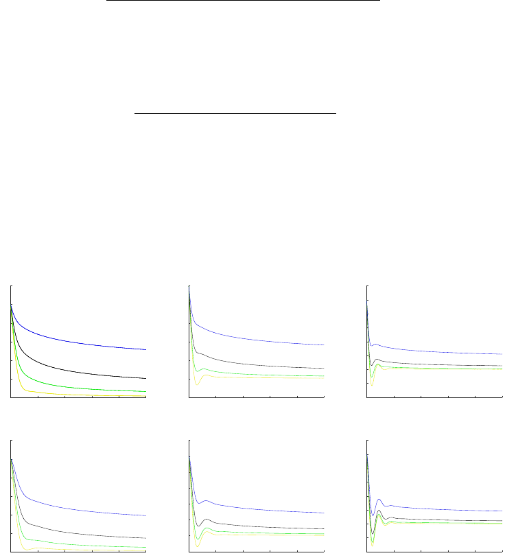
Paper E
·
Stochastic differential equations with a fractionally filtered delay: a semimartingale
model for long-range dependent processes
and this can only happen if
y
= 0, since
x, κ
1
,κ
2
>
0 and the sign of
y
is the same
as that of
sin
(
βθ
z
). However, if
y
= 0 it is easy to see that the real part of
(4.14)
cannot be zero for any
x >
0, so we conclude that
(4.3)
holds and that there exists a
stationary solution (
X
t
)
t∈R
given through the kernel
(4.4)
. With
γ
1
=
cos
(
βπ/
2) and
γ
2
= sin(βπ/2) the autocovariance function γ
X
is given by
γ
X
(t) =
Z
R
e
ity
y
2
+ κ
2
1
y
4
+ 2κ
2
κ
1
γ
2
|y|
1+β
−γ
1
|y|
2+β
+ κ
2
1
y
2
+ κ
2
2
|y|
2β
dy, t ∈ R. (4.15)
The polynomials to the associated FICARMA(2
,β,
1) process are given by
P
(
z
) =
z
2
+
κ
1
z
+
κ
2
and
Q
(
z
) =
z
+
κ
1
(see Remark 4.3) and the autocovariance function
γ
β
takes the form
γ
β
(t) =
Z
R
e
ity
y
2
+ κ
2
1
|y|
4+2β
+ (κ
2
1
−2κ
2
)|y|
2+2β
+ κ
2
2
|y|
2β
dy, t ∈ R. (4.16)
In Figure 2 we have plotted the ACF based on
(4.15)
for
κ
1
= 1 and various values of
κ
2
and
β
. For comparison we have also plotted the ACF based on
(4.16)
for the same
choices of
κ
1
,
κ
2
and
β
. From these plots we see that both the ACF corresponding to
(4.15)
and
(4.16)
are decreasing in
κ
2
, which is similar to the role of
κ
in Example 4.4.
It appears as well that a larger
κ
2
causes more curvature, although this effect is less
pronounced for (4.15) than for (4.16).
0 10 20 30 40 50
0
0.2
0.4
0.6
0.8
1
1.2
0 10 20 30 40 50
-0.2
0
0.2
0.4
0.6
0.8
1
0 10 20 30 40 50
-0.4
-0.2
0
0.2
0.4
0.6
0.8
1
1.2
0 10 20 30 40 50
0
0.2
0.4
0.6
0.8
1
1.2
0 10 20 30 40 50
-0.2
0
0.2
0.4
0.6
0.8
1
1.2
0 10 20 30 40 50
-0.4
-0.2
0
0.2
0.4
0.6
0.8
1
1.2
Figure 2:
First row is ACF based on
(4.15)
, second row is ACF based on
(4.16)
, and the columns correspond
to
κ
2
= 0
.
5,
κ
2
= 1 and
κ
2
= 2, respectively. Within each plot, the lines correspond to
β
= 0
.
1 (yellow),
β = 0.2 (green), β = 0.3 (black) and β = 0.4 (blue). In all plots, κ
1
= 1.
5 Simulation from the SFDDE
In the following we will focus on simulating from
(3.3)
. We begin this simulation
study by considering the Ornstein–Uhlenbeck type equation discussed in Example 4.4
120

5 · Simulation from the SFDDE
with
κ
= 1 and under the assumption that (
L
t
)
t∈R
is a standard Brownian motion. Let
c
1
=
100/∆
and
c
2
=
2000/∆
. We generate a simulation of the solution process (
X
t
)
t∈R
on a grid of size
∆
= 0
.
01 and with
3700/∆
steps of size
∆
starting from
−c
1
−c
2
and
ending at
1600/∆
. Initially, we set
X
t
equal to zero for the first
c
1
points in the grid
and then discretize (4.8) using the approximation
Z
R
h
(n∆ −u)
−β
+
−((n −1)∆ −u)
−β
+
i
X
u
du
'
1
1 −β
∆
1−β
X
(n−1)∆
+
n−1
X
k=n−c
1
X
k∆
+ X
(k−1)∆
2
Z
k∆
(k−1)∆
h
(n∆ −u)
−β
+
−((n −1)∆ −u)
−β
+
i
du
=
1
1 −β
∆
1−β
X
(n−1)∆
+
1
1 −β
n−1
X
k=n−c
1
X
k∆
+ X
(k−1)∆
2
·
2((n −k −1)∆)
1−β
−((n −k)∆)
1−β
−((n −k −2)∆)
1−β
for
n
=
−c
2
+ 1
,... ,
3700
/∆ − c
2
− c
1
. Next, we disregard the first
c
1
+
c
2
values of
the simulated sample path to obtain an approximate sample from the stationary
distribution. We assume that the process is observed on a unit grid resulting in
simulated values
X
1
,... , X
1600
. This is repeated
200
times, and in every repetition the
sample ACF based on
X
1
,... , X
L
is computed for
t
= 1
,... ,
25 and
L
=
100,400,1600
.
In long-memory models, the sample mean
¯
X
L
can be a poor approximation to the
true mean
E
[
X
0
] even for large
L
, and this may result in considerable negative (finite
sample) bias in the sample ACF (see, e.g., [23]). Due to this bias, it may be difficult to
see if we succeed in simulating from
(3.3)
, and hence we will assume that
E
[
X
0
] is
known to be zero when computing the sample ACF. We calculate the
95 %
confidence
interval
h
¯
ρ(k) −1.96
ˆ
σ(k)
√
200
,
¯
ρ(k) + 1.96
ˆ
σ(k)
√
200
i
,
for the mean of the sample ACF based on
L
observations at lag
k
. Here
¯
ρ
(
k
) is the
sample mean and
ˆ
σ
(
k
) is the sample standard deviations of the ACF at lag
k
based on
the
200
replications. In Figure 3, the theoretical ACFs and the corresponding
95 %
confidence intervals for the mean of the sample ACFs are plotted for
β
= 0
.
1
,
0
.
2 and
L
=
100,400,1600
. We see that, when correcting for the bias induced by an unknown
mean
E
[
X
0
], simulation from equation
(4.8)
results in a fairly unbiased estimator of
the ACF for small values of
β
. When
β >
0
.
25, in the case where the ACF of (
X
t
)
t∈R
is not even in
L
2
, the results are more unstable as it requires large values of
c
1
and
c
2
to ensure that the simulation results in a good approximation to the stationary
distribution of (
X
t
)
t∈R
. Moreover, even after correcting for the bias induced by an
unknown mean of the observed process, the sample ACF for the ARFIMA process
shows considerable finite sample bias when
β >
0
.
25, see [23], and hence we may
expect this to apply to solutions to (3.3) as well.
In Figure 4 we have plotted box plots for the 200 replications of the sample ACF
for
β
= 0
.
1
,
0
.
2 and
L
=
100,400,1600
. We see that the sample ACFs have the expected
convergence when
L
grows and that the distribution is more concentrated in the case
where less memory is present.
121

Paper E
·
Stochastic differential equations with a fractionally filtered delay: a semimartingale
model for long-range dependent processes
0 5 10 15 20 25
0
0.2
0.4
0.6
0.8
1
0 5 10 15 20 25
0
0.2
0.4
0.6
0.8
1
0 5 10 15 20 25
0
0.2
0.4
0.6
0.8
1
0 5 10 15 20 25
0
0.2
0.4
0.6
0.8
1
0 5 10 15 20 25
0
0.2
0.4
0.6
0.8
1
0 5 10 15 20 25
0
0.2
0.4
0.6
0.8
1
Figure 3:
Theoretical ACF and
95 %
confidence intervals of the mean of the sample ACF based on
200
replications of
X
1
,.. .,X
L
. Columns correspond to
L
=
100
,
L
=
400
and
L
=
1600
, respectively, and rows
correspond to β = 0.1 and β = 0.2, respectively. The model is (4.8).
0 5 10 15 20 25
-0.4
-0.2
0
0.2
0.4
0.6
0.8
1
0 5 10 15 20 25
-0.4
-0.2
0
0.2
0.4
0.6
0.8
1
0 5 10 15 20 25
-0.4
-0.2
0
0.2
0.4
0.6
0.8
1
0 5 10 15 20 25
-0.4
-0.2
0
0.2
0.4
0.6
0.8
1
0 5 10 15 20 25
-0.4
-0.2
0
0.2
0.4
0.6
0.8
1
0 5 10 15 20 25
-0.4
-0.2
0
0.2
0.4
0.6
0.8
1
Figure 4:
Box plots for the sample ACF based on
200
replications of
X
1
,.. .,X
L
together with the theoretical
ACF. Columns correspond to
L
=
100
,
L
=
400
and
L
=
1600
, respectively, and rows correspond to
β
= 0
.
1
and β = 0.2, respectively. The model is (4.8).
122

6 · Proofs
Following the same approach as above, we simulate the solution to the equation
discussed in Example 4.5. Specifically, the simulation is based on equation
(3.3)
,
restricted to the case where
η
(
dt
) =
−e
−t
dt
and (
L
t
)
t∈R
is a standard Brownian motion.
In this case, we use the approximation
Z
R
h
(n∆ −u)
−β
+
−((n −1)∆ −u)
−β
+
i
Z
∞
0
X
u−v
e
−v
dv du
=
Z
∞
0
X
n∆−v
Z
v
0
h
(u −∆)
−β
+
−u
−β
+
i
e
u−v
du dv
'
1
2
∆X
(n−1)∆
f (∆)
+
c
1
X
k=2
1
4
∆
X
(n−k)∆
+ X
(n−k+1)∆
ϕ(k∆) + ϕ((k −1)∆)
where ϕ : R → R is given by
ϕ(v) =
Z
v
0
h
(u −∆)
−β
+
−u
−β
i
e
u−v
du.
We approximate ϕ recursively by noting that
ϕ(k∆) =
Z
k∆
0
h
(u −∆)
−β
+
−u
−β
i
e
u−k∆
dv
'
1 + e
−∆
2
Z
k∆
(k−1)∆
h
(u −∆)
−β
+
−u
−β
+
i
dv + e
−∆
ϕ((k −1)∆)
=
1
1 −β
1 + e
−∆
2
h
((k −1)∆)
1−β
−(k∆)
1−β
i
+ e
−∆
ϕ((k −1)∆)
for
k ≥
1. The theoretical ACFs and corresponding
95 %
confidence intervals are
plotted in Figure 5 and the box plots in Figure 6. The findings are consistent with the
first example that we considered in the sense of convergence of the sample ACF and
the effect of memory (the value of β).
6 Proofs
Proof of Proposition 3.1.
For
γ >
0 define
h
γ
(
z
) =
z
γ
/h
(
z
) for each
z ∈ C \{
0
}
with
Re
(
z
)
≥
0. By continuity of
h
and the asymptotics
|h
γ
(
z
)
| ∼ |η
([0
,∞
))
|
−1
|z|
γ
,
|z| →
0,
and |h
γ
(z)| ∼ |z|
γ−1
, |z| → ∞, it follows that
sup
x>0
Z
R
|h
γ
(x + iy)|
2
dy < ∞ (6.1)
for
γ ∈
(
−
1
/
2
,
1
/
2). In other words,
h
γ
is a certain Hardy function, and thus there exists
a function
f
γ
: R → R
in
L
2
which is vanishing on (
−∞,
0) and has
L
[
f
γ
](
z
) =
h
γ
(
z
)
when
Re
(
z
)
>
0, see [2, 11, 13]. Note that
f
γ
is indeed real-valued, since
h
γ
(x −iy)
=
h
γ
(
x
+
iy
) for
y ∈ R
and a fixed
x >
0. We can apply [24, Proposition 2.3] to deduce
that there exists a function
g ∈ L
2
satisfying
(3.6)
and that it can be represented as
the (left-sided) Riemann–Liouville fractional integral of f
0
, that is,
g(t) =
1
Γ (β)
Z
t
0
f
0
(u)(t −u)
β−1
du, t > 0.
123

Paper E
·
Stochastic differential equations with a fractionally filtered delay: a semimartingale
model for long-range dependent processes
0 5 10 15 20 25
-0.2
0
0.2
0.4
0.6
0.8
1
0 5 10 15 20 25
-0.2
0
0.2
0.4
0.6
0.8
1
0 5 10 15 20 25
-0.2
0
0.2
0.4
0.6
0.8
1
0 5 10 15 20 25
-0.2
0
0.2
0.4
0.6
0.8
1
0 5 10 15 20 25
-0.2
0
0.2
0.4
0.6
0.8
1
0 5 10 15 20 25
-0.2
0
0.2
0.4
0.6
0.8
1
Figure 5:
Theoretical ACF and
95 %
confidence intervals of the mean of the sample ACF sample based
on
200
replications of
X
1
,.. .,X
L
. Columns correspond to
L
=
100
,
L
=
400
and
L
=
1600
, respectively, and
rows correspond to β = 0.1 and β = 0.2, respectively. The model is (4.13).
0 5 10 15 20 25
-0.4
-0.2
0
0.2
0.4
0.6
0.8
1
0 5 10 15 20 25
-0.4
-0.2
0
0.2
0.4
0.6
0.8
1
0 5 10 15 20 25
-0.4
-0.2
0
0.2
0.4
0.6
0.8
1
0 5 10 15 20 25
-0.4
-0.2
0
0.2
0.4
0.6
0.8
1
0 5 10 15 20 25
-0.4
-0.2
0
0.2
0.4
0.6
0.8
1
0 5 10 15 20 25
-0.4
-0.2
0
0.2
0.4
0.6
0.8
1
Figure 6:
Box plots for the sample ACF based on
200
replications of
X
1
,.. .,X
L
together with the theoretical
ACF. Columns correspond to
L
=
100
,
L
=
400
and
L
=
1600
, respectively, and rows correspond to
β
= 0
.
1
and β = 0.2, respectively. The model is (4.13).
124

6 · Proofs
Conversely, [24, Theorem 2.1] ensures that
D
β
g
given by
(3.7)
is a well-defined limit
and that
D
β
g
=
f
0
. In particular, we have shown (ii) and if we can argue that
f
0
∈ L
1
,
we have shown (i) as well. This follows from the assumption in
(3.1)
, since then we
have that
y 7→ L
[
f
0
](
x
+
iy
) is differentiable for any
x ≥
0 (except at 0 when
x
= 0) and
L[u 7→ uf
0
(u)](x + iy) = i
d
dy
L[f
0
](x + iy)
=
L[u η(du)](x + iy) + (1 −β)(x + iy)
−β
h(x + iy)
2
.
(6.2)
The function
L
[
u 7→ uf
0
(
u
)] is analytic on
{z ∈ C
:
Re
(
z
)
<
0
}
and from the identity
(6.2)
it is not too difficult to see that it also satisfies the Hardy condition
(6.1)
. This
means
u 7→ uf
0
(
u
) belongs to
L
2
, and hence we have that
f
0
belongs to
L
1
. Since
g
is
the Riemann–Liouville integral of
f
0
of order
β
and
f
0
∈ L
1
∩L
2
, [3, Proposition 4.3]
implies that g ∈ L
γ
for (1 −β)
−1
< γ ≤ 2.
It is straightforward to verify (3.9) and to obtain the identity
Z
t
s
D
β
g
∗η(u − · ) du =
Z
R
D
β
−
1
(s,t]
(u)g ∗η(u − · ) du
almost everywhere by comparing their Fourier transforms. This establishes the rela-
tion
g(t −v) −g(s −v) =
Z
t
s
D
β
g
∗η(u −v) du + 1
(s,t]
(v).
By letting
s → −∞
, and using that
D
β
g
and
g
are both vanishing on (
−∞,
0), we deduce
that
g(t) = 1
[0,∞)
(t)
1 +
Z
t
0
D
β
g
∗η(u) du
,
for almost all t ∈ R which shows (3.8) and, thus, finishes the proof.
Proof of Theorem 3.2.
Since
g ∈L
2
, according to Proposition 3.1, and
E
[
L
2
1
]
< ∞
and
E[L
1
] = 0,
X
t
=
Z
t
−∞
g(t −u) dL
u
, t ∈ R,
is a well-defined process (e.g., in the sense of [26]) which is stationary with mean zero
and finite second moments. By integrating both sides of
(3.9)
with respect to (
L
t
)
t∈R
we obtain
X
t
−X
s
=
Z
R
Z
R
D
β
−
1
(s,t]
(u)g ∗η(u −r) du
dL
r
+ L
t
−L
s
.
By a stochastic Fubini result (e.g., [1, Theorem 3.1]) we can change the order of
integration (twice) and obtain
Z
R
Z
R
D
β
−
1
(s,t]
(u)g ∗η(u −r) du
dL
r
=
Z
R
D
β
−
1
(s,t]
(u)X ∗η(u) du.
This shows that (
X
t
)
t∈R
is a solution to
(3.3)
. To show uniqueness, note that the spec-
tral process
Λ
X
(with spectral distribution, say,
F
X
) of any purely non-deterministic
solution (X
t
)
t∈R
satisfies
Z
R
F [1
(s,t]
](−y)(iy)
β
h(iy)Λ
X
(dy) = L
t
−L
s
(6.3)
125

Paper E
·
Stochastic differential equations with a fractionally filtered delay: a semimartingale
model for long-range dependent processes
almost surely for all choices of
s < t
. This follows from the results in the supplemen-
tary material on spectral representations (see Section 7). Using the fact that (
X
t
)
t∈R
is
purely non-deterministic,
F
X
is absolutely continuous with respect to the Lebesgue
measure, and hence we can extend
(6.3)
from
1
(s,t]
to any function
f ∈ L
2
using an
approximation of
f
with simple functions of the form
s
=
P
n
j=1
α
j
1
(t
j−1
,t
j
]
for
α
j
∈ C
and t
0
< t
1
< ··· < t
n
. Specifically, we establish that
Z
R
F [f ](−y)(iy)
β
h(iy)Λ
X
(dy) =
Z
R
f (u) dL
u
(6.4)
almost surely for any
f ∈ L
2
. In particular we may take
f
=
g
(
t − ·
),
g
being the
solution kernel characterized in
(3.6)
, so that
F
[
f
](
y
) =
e
−ity
(
−iy
)
−β
/h
(
−iy
) and
(6.4)
thus implies that X
t
=
R
t
−∞
g(t −u) dL
u
, which ends the proof.
Proof of Proposition 3.6.
We start by arguing that the limit in
(3.13)
exists and is
equal to
R
t
−∞
D
β
g
(
t −u
)
dL
u
. For a given
δ >
0 it follows by a stochastic Fubini result
that
β
Γ (1 −β)
Z
∞
δ
X
t
−X
t−u
u
1+β
du =
Z
R
D
β
δ
g(t −r) dL
r
, (6.5)
where
D
β
δ
g(t) =
β
Γ (1 −β)
Z
∞
δ
g(t) −g(t −u)
u
1+β
du, t > 0,
and
D
β
δ
g
(
t
) = 0 for
t ≤
0. Suppose for the moment that (
L
t
)
t∈R
is a Brownian motion,
so that (
X
t
)
t∈R
is
γ
-Hölder continuous for all
γ ∈
(0
,
1
/
2) by
(3.3)
. Then, almost surely,
u 7→ (X
t
−X
t−u
)/u
1+β
is in L
1
and the relation (6.5) thus shows that
Z
R
h
D
β
δ
g(t −r) −D
β
δ
0
g(t −r)
i
dL
r
P
−−→ 0 as δ,δ
0
→ 0,
which in turn implies that (
D
β
δ
g
)
δ>0
has a limit in
L
2
. We also know that this limit
must be
D
β
g
, since
D
β
δ
g → D
β
g
pointwise as
δ ↓
0 by
(3.7)
. Having established this
convergence, which does not rely on (
L
t
)
t∈R
being a Brownian motion, it follows
immediately from
(6.5)
and the isometry property of the integral map
R
R
· dL
that
the limit in
(3.13)
exists and that
D
β
X
t
=
R
t
−∞
D
β
g
(
t−u
)
dL
u
. To show
(3.14)
we start by
recalling the definition of
D
β
−
1
(s,t]
in
(3.2)
and that
F
[
D
β
−
1
(s,t]
](
y
) = (
−iy
)
β
F
[
1
(s,t]
](
y
).
This identity can be shown by using that the improper integral
R
∞
0
e
±iv
v
γ−1
dv
is equal
to Γ (γ)e
±iπγ/2
for any γ ∈ (0, 1). Now observe that
F
Z
R
D
β
−
1
(s,t]
(u)g ∗η(u − · ) du
(y) = (−iy)
β
F [1
(s,t]
](y)F [g](−y)F [η](−y)
= F [1
(s,t]
](y)F
h
D
β
g
∗η
i
(−y)
= F
Z
t
s
D
β
g
∗η(u − · ) du
(y),
and hence
R
R
(
D
β
−
1
(s,t]
)(
u
)
g ∗η
(
u − ·
)
du
=
R
t
s
(
D
β
g
)
∗η
(
u − ·
)
du
almost everywhere.
Consequently, using that
D
β
X
t
=
R
t
−∞
D
β
g
(
t −u
)
dL
u
and applying a stochastic Fubini
126

6 · Proofs
result twice,
Z
t
s
D
β
X
∗η(u) du =
Z
R
Z
t
s
D
β
g
∗η(u −r) du dL
r
=
Z
R
Z
R
D
β
−
1
(s,t]
(u)g ∗η(u −r) du dL
r
=
1
Γ (1 −β)
Z
R
h
(t −u)
−β
+
−(s −u)
−β
+
i
X ∗η(u) du.
The semimartingale property of (
X
t
)
t∈R
is now an immediate consequence of
(3.3)
.
Proof of Proposition 3.7.
Using
(3.16)
and that
h
(0) =
−η
([0
,∞
)), it follows that
f
X
(
y
)
∼ |y|
−2β
/η
([0
,∞
))
2
as
y →
0. To show the asymptotic behavior of
γ
X
at
∞
we
start by recalling that, for u, v ∈ R,
Z
∞
u∨v
(s −u)
β−1
(s −v)
β−1
ds =
Γ (β)Γ (1 −2β)
Γ (1 −β)
|u −v|
2β−1
by [16, p. 404]. Having this relation in mind we use Proposition 3.1(ii) and
(3.15)
to
do the computations
γ
X
(t) =
1
Γ (β)
2
Z
R
Z
R
Z
R
D
β
g(u)D
β
g(v)(s + t −u)
β−1
+
(s −v)
β−1
+
dv du ds
=
1
Γ (β)
2
Z
R
Z
R
D
β
g(u)D
β
g(v)
·
Z
∞
(u−t)∨v
(s −(u −t))
β−1
(s −v)
β−1
ds dv du
=
Γ (1 −2β)
Γ (β)Γ (1 −β)
Z
R
Z
R
D
β
g(u)D
β
g(v)|u −v −t|
2β−1
dv du
=
Γ (1 −2β)
Γ (β)Γ (1 −β)
Z
R
γ(u)|u −t|
2β−1
du, (6.6)
where
γ
(
u
) =
R
R
D
β
g
(
u
+
v
)
D
β
g
(
v
)
dv
. Note that
γ ∈ L
1
since
D
β
g ∈ L
1
by Proposi-
tion 3.1 and, using Plancherel’s theorem,
γ(u) =
Z
R
e
−iuy
F [D
β
g](y)
2
dy = F [|h(i · )|
−2
](u).
In particular
R
R
γ
(
u
)
du
=
|h
(0)
|
−2
=
η
([0
,∞
))
−2
, and hence it follows from
(6.6)
that
we have shown the result if we can argue that
R
R
γ(u)|u −t|
2β−1
du
t
2β−1
=
Z
R
γ(u)
|
u
t
−1|
1−2β
du →
Z
R
γ(u) du as t → ∞. (6.7)
It is clear by Lebesgue’s theorem on dominated convergence that
Z
0
−∞
γ(u)
|
u
t
−1|
1−2β
du →
Z
0
−∞
γ(u) du as t → ∞.
Moreover, since
|h
(
i ·
)
|
−2
is continuous at 0 and differentiable on (
−∞,
0) and (0
,∞
)
with integrable derivatives, it is absolutely continuous on
R
with a density
φ
in
L
1
.
127

Paper E
·
Stochastic differential equations with a fractionally filtered delay: a semimartingale
model for long-range dependent processes
As a consequence, γ(u) = F [φ](u)/(iu) and, thus,
Z
∞
t/2
γ(u)
|
u
t
−1|
1−2β
du =
Z
∞
1/2
tγ(tu)
|u −1|
1−2β
du = −i
Z
∞
1/2
F [φ](tu)
u|u −1|
1−2β
du. (6.8)
By the Riemann–Lebesgue lemma and Lebesgue’s theorem on dominated convergence
it follows that the right-hand side of expression in
(6.8)
tends to zero as
t
tends to
infinity. Finally, integration by parts and the symmetry of γ yields
Z
t/2
0
γ(u)
1 −
1
|
u
t
−1|
1−2β
du =
Z
1/2
0
tγ(tu)
1 −
1
(1 −u)
1−2β
du
=
2
1−2β
−1
Z
−t/2
−∞
γ(u) du
−
Z
1/2
0
1 −2β
(1 −u)
2−2β
Z
−tu
−∞
γ(v) dv du,
where both terms on the right-hand side converge to zero as
t
tends to infinity. Thus,
we have shown (6.7), and this completes the proof.
Proof of Proposition 3.8.
Observe that it is sufficient to argue
E
[(
X
t
−X
0
)
2
]
∼ t
as
t ↓
0. By using the spectral representation
X
t
=
R
R
e
ity
Λ
X
(
dy
) and the isometry prop-
erty of the integral map
R
R
· dΛ
X
: L
2
(F
X
) → L
2
(P), see [15, p. 389], we have that
E[(X
t
−X
0
)
2
]
t
= t
−2
Z
R
|1 −e
iy
|
2
f
X
(y/t) dy
=
Z
R
|1 −e
iy
|
2
|y|
2β
|(iy)
1−β
−t
1−β
F [η](y/t)|
2
dy. (6.9)
Consider now a
y ∈ R
satisfying
|y|≥ C
1
t
with
C
1
B
(2
|η|
([0
,∞
)))
1/(1−β)
. In this case
|y|
1−β
/
2
−|t
1−β
F
[
η
](
y/t
)
| ≥
0, and we thus get by the reversed triangle inequality that
|1 −e
iy
|
2
|y|
2β
|(iy)
1−β
−t
1−β
F [η](y/t)|
2
≤ 2
|1 −e
iy
|
2
y
2
.
If |y|< C
1
t, we note that the assumption on the function in (3.5) implies that
C
2
B inf
|x|≤C
1
(ix)
1−β
−F [η](x)
> 0,
which shows that
(iy)
1−β
−t
1−β
F [η](y/t)
≥ t
1−β
C
2
≥
C
2
C
1−β
1
|y|
1−β
.
This establishes that
|1 −e
iy
|
2
|y|
2β
(iy)
1−β
−t
1−β
F [η](y/t)
2
≤
C
2(1−β)
1
C
2
2
|1 −e
iy
|
2
y
2
.
Consequently, it follows from
(6.9)
and Lebesgue’s theorem on dominated conver-
gence that
E[(X
t
−X
0
)
2
]
t
→
Z
R
|1 −e
iy
|
2
y
2
dy =
Z
R
|F [1
(0,1]
](y)|
2
dy = 1 as t ↓ 0,
which was to be shown.
128

6 · Proofs
Proof of Proposition 3.11.
We start by arguing that the first term on the right-hand
side of the formula is well-defined. In order to do so it suffices to argue that
E
Z
t−s
0
Z
s
−∞
|X
w
|
Z
[0,∞)
D
β
−
1
(s,t−u]
(v + w)
|η|(dv) dw |g|(du)
≤ E[|X
0
|]
Z
t−s
0
Z
[0,∞)
Z
s
−∞
D
β
−
1
(s,t−u]
(v + w)
dw |η|(dv)|g|(du)
(6.10)
is finite. This is implied by the facts that
Γ (1 −β)
Z
s
−∞
D
β
−
1
(s,t−u]
(v + w)
dw
≤
Z
0
u+s−t
(t −s −u + w)
−β
dw +
Z
1
0
h
w
−β
−(t −s −u + w)
−β
i
dw
+ (1 + β)
Z
∞
1
w
−1−β
(t −s −u) dw
=
1
1 −β
2(t −s −u)
1−β
+ 1 −(t −s −u + 1)
1−β
+
(1 + β)
β
(t −s −u)
≤
2
1 −β
(t −s)
1−β
+
(1 + β)
β
(t −s)
for
u ∈
[0
,t −s
] and
g
(
du
) is a finite measure (since
D
β
g ∈L
1
by Proposition 3.1). Now
fix an arbitrary z ∈ C with Re(z) > 0. It follows from (3.3) that
L[X1
(s,∞)
](z) = X
s
L[1
(s,∞
](z) + L[1
(s,∞)
(L
·
−L
s
)](z)
+ L
h
1
(s,∞)
Z
R
X
u
Z
[0,∞)
D
β
−
1
(s, · ]
(u + v)η(dv) du
i
(z).
(6.11)
By noting that (D
β
−
1
(s,t]
)(u) = 0 when t ≤ s < u we obtain
L
h
1
(s,∞)
Z
∞
s
X
u
Z
[0,∞)
D
β
−
1
(s, · ]
(u + v)η(dv) du
i
(z)
=
1
Γ (1 −β)
L
Z
∞
s
X
u
Z
[0,∞)
( · −u −v)
−β
+
η(dv) du
(z)
= L[1
(s,∞)
X](z)L[η](z)z
β−1
.
Combining this observation with (6.11) we get the relation
z −z
β
L[η](z)
L[1
(s,∞)
X](z)
= zX
s
L[1
(s,∞)
](z) + zL[1
(s,∞)
(L −L
s
)](z)
+ zL
h
1
(s,∞)
Z
s
−∞
X
u
Z
[0,∞)
D
β
−
1
(s, · ]
(u + v)η(dv) du
i
(z),
129

Paper E
·
Stochastic differential equations with a fractionally filtered delay: a semimartingale
model for long-range dependent processes
which implies
L[1
(s,∞)
X](z)
= L[g](z)L[X
s
δ
0
(s − · )](z) + zL[g](z)L[1
(s,∞)
(L −L
s
)](z)
+ zL[g](z)L
h
1
(s,∞)
Z
s
−∞
X
u
Z
[0,∞)
D
β
−
1
(s, · ]
(u + v)η(dv) du
i
(z)
= L[g( · −s)X
s
](z) + L
Z
·
s
g( · −u)dL
u
(z)
+ L
Z
· −s
0
Z
s
−∞
X
w
Z
[0,∞)
D
β
−
1
(s, · −u]
(v + w)η(dv) dwg(du)
(z).
This establishes the identity
X
t
= g(t −s)X
s
+
Z
t
s
g(t −u) dL
u
+
Z
t−s
0
Z
s
−∞
X
w
Z
[0,∞)
D
β
−
1
(s,t−u]
(v + w)η(dv) dwg(du)
(6.12)
almost surely for Lebesgue almost all
t > s
. Since both sides of
(6.12)
are continuous
in
L
1
(
P
), the identity holds for each fixed pair
s < t
almost surely as well. By applying
the conditional mean E[ · | X
u
, u ≤ s] on both sides of (6.12) we obtain the result.
Proof of Corollary 4.1.
In this setup it follows that the function
h
in
(3.5)
is given by
h(z) = z
1−β
+ κ +
R(z)
Q(z)
,
where
Q
(
z
)
,
0 whenever
Re
(
z
)
≥
0 by the assumption on
A
. This shows that
h
is
non-zero (on {z ∈ C : Re(z) ≥ 0}) if and only if
Q(z)[z
1−β
+ κ] + R(z) , 0 for all z ∈ C with Re(z) ≥ 0. (6.13)
Condition
(6.13)
may equivalently be formulated as
Q
(
z
)[
z
+
κz
β
] +
R
(
z
)
z
β
,
0 for all
z ∈ C \{
0
}
with
Re
(
z
)
≥
0 and
h
(0) =
κ
+
b
>
A
−1
e
1
,
0, which by Theorem 3.2 shows
that a unique solution to
(4.5)
exists. It also provides the form of the solution, namely
(3.11) with
F [g](y) =
(iy)
−β
(iy)
1−β
+ κ +
R(iy)
Q(iy)
=
Q(iy)
Q(iy)[iy + κ(iy)
β
] + R(iy)(iy)
β
, y ∈ R.
This finishes the proof.
Proof of Proposition 4.2.
We will first show that
D
β
f ∈ L
1
. By using that
R
∞
0
e
Au
du
=
−A
−1
we can rewrite D
β
f as
D
β
f (t) =
1
Γ (1 −β)
b
>
A
Z
t
0
e
Au
h
(t −u)
−β
−t
−β
i
du −
Z
∞
t
e
Au
t
−β
du
e
1
, t > 0,
from which we see that it suffices to argue that (each entry of)
t 7−→
Z
t
0
e
Au
h
(t −u)
−β
−t
−β
i
du
130

7 · Supplement
belongs to
L
1
. Since
u 7→ e
Au
is continuous and with all entries decaying exponentially
fast as u → ∞, this follows from the fact that, for a given γ > 0,
Z
∞
0
Z
t
0
e
−γu
(t −u)
−β
−t
−β
du dt
≤
Z
∞
0
e
−γu
Z
u+1
u
h
(t −u)
−β
+ t
−β
i
dt + βu
Z
∞
1
t
−β−1
dt
du < ∞.
Here we have used the mean value theorem to establish the inequality
(t −u)
−β
−t
−β
≤ βu(t −u)
−β−1
for 0
< u < t
. To show that
D
β
f ∈ L
2
, note that it is the left-sided Riemann–Liouville
fractional derivative of f , that is,
D
β
f (t) =
1
Γ (1 −β)
d
dt
Z
t
0
f (t −u)u
−β
du, t > 0.
Consequently, it follows by [27, Theorem 7.1] that the Fourier transform
F
[
D
β
f
] of
f is given by
F [D
β
f ](y) = (iy)
β
F [f ](y) = (iy)
β
b
>
(iy −A)
−1
e
1
, y ∈ R,
in particular it belongs to
L
2
(e.g., by Cramer’s rule), and thus
D
β
f ∈ L
2
. By comparing
Fourier transforms we establish that (D
β
g) ∗f = g ∗(D
β
f ), and hence it holds that
Z
∞
0
D
β
X
t−u
f (u) du =
Z
R
D
β
g
∗f (t −r) dL
r
=
Z
∞
0
X
t−u
D
β
f (u) du
using Proposition 3.6 and a stochastic Fubini result. This finishes the proof.
7 Supplement to “Stochastic differential equations with a
fractionally filtered delay: a semimartingale model for
long-range dependent processes”
This supplement provides an exposition of the spectral representation and related
results for continuous-time stationary, measurable, centered and square integrable
processes. The content of the results should be well-known and is mainly provided
for reference.
7.1 Spectral representations of continuous-time stationary processes
In the following we present and prove a few results related to the spectral theory for
continuous-time stationary, measurable, centered and square integrable processes.
Although the results should be well-known, we have not been able to find an appro-
priate reference to earlier literature. However, the results presented here rely heavily
on [15, Section 9.4] and [20, Appendix A2.1], in which an extensive treatment of the
spectral theory is given.
Recall that if S = {S(t) : t ∈ R} is a (complex-valued) process such that
(i) E[|S(t)|
2
] < ∞ for all t ∈ R,
131

Paper E
·
Stochastic differential equations with a fractionally filtered delay: a semimartingale
model for long-range dependent processes
(ii) E[|S(t + s) −S(t)|
2
] → 0 as s ↓ 0 for all t ∈ R, and
(iii) E[(S(v) −S(u))(S(t) −S(s))] = 0 for all u ≤ v ≤s ≤ t,
we may (and do) define integration of
f
with respect to
S
in the sense of [15, pp.
388–390] for any f ∈ L
2
(G), where G is the control measure characterized by
G((s,t]) = E[|S(t) −S(s)|
2
], s < t.
We have the following stochastic Fubini result for this type of integral:
Proposition 7.1.
Let
S
=
{S
(
t
) :
t ∈ R}
be a process given as above. Let
µ
be a finite Borel
measure on
R
, and let
f : R
2
→ C
be a measurable function in
L
2
(
µ ×G
). Then all the
integrals below are well-defined and
Z
R
Z
R
f (x,y)µ(dx)
S(dy) =
Z
R
Z
R
f (x,y)S(dy)
µ(dx) (7.1)
almost surely.
Suppose that (
X
t
)
t∈R
is a measurable and stationary process with
E
[
X
2
0
]
< ∞
and
E
[
X
0
] = 0, and denote by
γ
X
its autocovariance function. Since (
X
t
)
t∈R
is continuous
in
L
2
(
P
) (cf. [1, Corollary A.3]), it follows by Bochner’s theorem that there exists a
finite Borel measure F
X
on R such that
γ
X
(t) =
Z
R
e
ity
F
X
(dy), t ∈ R.
The measure F
X
is referred to as the spectral distribution of (X
t
)
t∈R
.
Theorem 7.2.
Let (
X
t
)
t∈R
be given as above and let
F
X
be the associated spectral distribu-
tion. Then there exists a (complex-valued) process
Λ
X
=
{Λ
X
(
y
) :
y ∈ R}
satisfying (i)–(iii)
above with control measure F
X
, such that
X
t
=
Z
R
e
ity
Λ
X
(dy) (7.2)
almost surely for each
t ∈ R
. The process
Λ
X
is called the spectral process of (
X
t
)
t∈R
and
(7.2) is referred to as its spectral representation.
Remark 7.3.
Let the situation be as in Theorem 7.2 and note that if there exists
another process
˜
Λ
X
= {
˜
Λ
X
(y) : y ∈ R} such that
X
t
=
Z
R
e
ity
˜
Λ
X
(dy), t ∈ R,
then its control measure is necessarily given by F
X
and
Z
R
f (y)Λ
X
(dy) =
Z
R
f (y)
˜
Λ
X
(dy)
almost surely for all f ∈L
2
(F
X
).
132

7 · Supplement
Proof of Proposition 7.1.
First, note that
(7.1)
is trivially true when
f
is of the form
f (x,y) =
n
X
j=1
α
j
1
A
j
(x)1
B
j
(y) (7.3)
for
α
1
,... , α
n
∈ C
and Borel sets
A
1
,B
1
,... , A
n
,B
n
⊆ R
. Now consider a general
f ∈
L
2
(
µ × G
) and choose a sequence of functions (
f
n
)
n∈N
of the form
(7.3)
such that
f
n
→ f in L
2
(µ ×G) as n → ∞. Set
X
n
=
Z
R
Z
R
f
n
(x, y)µ(dx)
S(dy), X =
Z
R
Z
R
f (x,y)µ(dx)
S(dy)
and Y =
Z
R
Z
R
f (x,y)S(dy)
µ(dx)
Observe that
X
and
Y
are indeed well-defined, since
x 7→ f
(
x, y
) is in
L
1
(
µ
) for
G
-
almost all y, y 7→ f (x,y) is in L
2
(G) for µ-almost all x,
Z
R
Z
R
f (x,y)µ(dx)
2
G(dy) ≤µ(R)
Z
R
2
|f (x,y)|
2
(µ ×G)(dx,dy) < ∞
and E
Z
R
Z
R
f (x,y)S(dy)
2
µ(dx)
=
Z
R
2
|f (x,y)|
2
(µ ×G)(dx,dy) < ∞.
Next, we find that
E[|X −X
n
|
2
] =
Z
R
Z
R
(f (x,y) −f
n
(x, y))µ(dx)
2
G(dy)
≤ µ(R)
Z
R
2
|f (x,y) −f
n
(x, y)|
2
(µ ×G)(dx,dy)
which tends to zero by the choice of (
f
n
)
n∈N
. Since
X
n
=
R
R
R
R
f
n
(x, y)S(dy)
µ
(
dx
), one
shows in a similar way that
X
n
→ Y
in
L
2
(
P
), and hence we conclude that
X
=
Y
almost surely.
Proof of Theorem 7.2.
For any given
t ∈ R
set
f
t
(
y
) =
e
ity
,
y ∈ R
, and let
H
F
and
H
X
be the set of all (complex) linear combinations of
{f
t
:
t ∈ R}
and
{X
t
:
t ∈ R}
,
respectively. By equipping
H
F
and
H
X
with the usual inner products on
L
2
(
F
X
) and
L
2
(P), their closures H
F
and H
X
are Hilbert spaces. Due to the fact that
hX
s
,X
t
i
L
2
(P)
= E[X
s
X
t
] =
Z
R
e
i(t−s)x
F
X
(dy) = hf
s
,f
t
i
L
2
(F
X
)
, s,t ∈ R,
we can define a linear isometric isomorphism µ: H
F
→ H
X
as the one satisfying
µ
n
X
j=1
α
j
f
t
j
=
n
X
j=1
α
j
X
t
j
for any given
n ∈ N
,
α
1
,... , α
n
∈ C
and
t
1
< ··· < t
n
. Since
1
(−∞,y]
∈ H
F
for each
y ∈ R
(cf. [32, p. 150]), we can associate a complex-valued process
Λ
X
=
{Λ
X
(
y
) :
y ∈ R}
to
(X
t
)
t∈R
through the relation
Λ
X
(y) = µ(1
(−∞,y]
), y ∈ R.
133

Paper E
·
Stochastic differential equations with a fractionally filtered delay: a semimartingale
model for long-range dependent processes
It is straight-forward to check from the isometry property that
Λ
X
is right-continuous
in L
2
(P), has orthogonal increments and satisfies
E[|Λ
X
(y
2
) −Λ
X
(y
1
)|
2
] = F
X
((y
1
,y
2
]), y
1
< y
2
.
Consequently, integration with respect to
Λ
X
of any function
f ∈ L
2
(
F
X
) can be
defined in the sense of [15, pp. 388–390]. For any
n ∈ N
,
α
1
,... , α
n
∈ C
and
t
0
< t
1
<
···< t
n
, we have
Z
R
n
X
j=1
α
j
1
(t
j−1
,t
j
]
(y)
Λ
X
(dy) =
n
X
j=1
α
j
µ(1
(t
j−1
,t
j
]
) = µ
n
X
j=1
α
j
1
(t
j−1
,t
j
]
.
Since
f 7→
R
R
f
(
y
)
Λ
X
(
dy
) is a continuous map (from
L
2
(
F
X
) into
L
2
(
P
)), it follows by
approximation with simple functions and from the relation above that
Z
R
f (y)Λ
X
(dy) = µ(f )
almost surely for any f ∈ H
F
. In particular, it shows that
X
t
= µ(f
t
) =
Z
R
e
ity
Λ
X
(dy), t ∈ R,
which is the spectral representation of (X
t
)
t∈R
.
Acknowledgments
The authors thank Andreas Basse-O’Connor and Jan Pedersen for helpful comments.
The research of Richard Davis was supported in part by ARO MURI grant W911NF–
12–1–0385. The research of Mikkel Slot Nielsen and Victor Rohde was supported by
Danish Council for Independent Research grant DFF–4002–00003.
References
[1]
Barndorff-Nielsen, O.E. and A. Basse-O’Connor (2011). Quasi Ornstein–Uhlen-
beck processes. Bernoulli 17(3), 916–941. doi: 10.3150/10-BEJ311.
[2]
Basse-O’Connor, A., M.S. Nielsen, J. Pedersen and V. Rohde (2019). Stochastic
delay differential equations and related autoregressive models. Stochastics.
Forthcoming. doi: 10.1080/17442508.2019.1635601.
[3]
Basse-O’Connor, A., M.S. Nielsen, J. Pedersen and V. Rohde (2018). Multivariate
stochastic delay differential equations and CAR representations of CARMA
processes. Stochastic Process. Appl. Forthcoming. doi:
10.1016/j.spa.2018.11
.011.
[4]
Bennedsen, M. (2015). Rough electricity: a new fractal multi-factor model of
electricity spot prices. CREATES Research Paper 42.
[5]
Bennedsen, M., A. Lunde and M.S. Pakkanen (2016). Decoupling the short-
and long-term behavior of stochastic volatility. arXiv: 1610.00332.
134
References
[6]
Beran, J., Y. Feng, S. Ghosh and R. Kulik (2016). Long-Memory Processes. Springer.
[7]
Bichteler, K. (1981). Stochastic integration and
L
p
-theory of semimartingales.
Ann. Probab. 9(1), 49–89.
[8]
Brockwell, P.J. and R.A. Davis (2006). Time series: theory and methods. Springer
Series in Statistics. Reprint of the second (1991) edition. Springer, New York.
[9]
Brockwell, P.J. and T. Marquardt (2005). Lévy-driven and fractionally inte-
grated ARMA processes with continuous time parameter. Statist. Sinica 15(2),
477–494.
[10]
Delbaen, F. and W. Schachermayer (1994). A general version of the fundamental
theorem of asset pricing. Math. Ann. 300(3), 463–520.
[11]
Doetsch, G. (1937). Bedingungen für die Darstellbarkeit einer Funktion als
Laplace-integral und eine Umkehrformel für die Laplace-Transformation. Math.
Z. 42(1), 263–286. doi: 10.1007/BF01160078.
[12]
Doukhan, P., G. Oppenheim and M.S. Taqqu, eds. (2003). Theory and applica-
tions of long-range dependence. Boston, MA: Birkhäuser Boston Inc.
[13]
Dym, H. and H.P McKean (1976). Gaussian processes, function theory, and the
inverse spectral problem. Probability and Mathematical Statistics, Vol. 31. New
York: Academic Press [Harcourt Brace Jovanovich Publishers].
[14]
Granger, C.W. and R. Joyeux (1980). An introduction to long-memory time
series models and fractional differencing. J. Time Series Anal. 1(1), 15–29.
[15]
Grimmett, G. and D. Stirzaker (2001). Probability and random processes. Oxford
University Press.
[16]
Gripenberg, G. and I. Norros (1996). On the prediction of fractional Brownian
motion. J. Appl. Probab. 33(2), 400–410.
[17]
Gushchin, A.A. and U. Küchler (2000). On stationary solutions of delay dif-
ferential equations driven by a Lévy process. Stochastic Process. Appl. 88(2),
195–211. doi: 10.1016/S0304-4149(99)00126-X.
[18] Hosking, J.R. (1981). Fractional differencing. Biometrika 68(1), 165–176.
[19]
Jusselin, P. and M. Rosenbaum (2018). No-arbitrage implies power-law market
impact and rough volatility. arXiv: 1805.07134.
[20] Koopmans, L.H. (1995). The spectral analysis of time series. Academic Press.
[21]
Marquardt, T. (2006). Fractional Lévy processes with an application to long
memory moving average processes. Bernoulli 12(6), 1099–1126.
[22]
Mohammed, S.E.A. and M.K.R. Scheutzow (1990). Lyapunov exponents and
stationary solutions for affine stochastic delay equations. Stochastics Stochastics
Rep. 29(2), 259–283.
[23]
Newbold, P. and C. Agiakloglou (1993). Bias in the sample autocorrelations of
fractional noise. Biometrika 80(3), 698–702.
135
Paper E
·
Stochastic differential equations with a fractionally filtered delay: a semimartingale
model for long-range dependent processes
[24]
Pipiras, V. and M.S. Taqqu (2003). Fractional calculus and its connections to
fractional Brownian motion. Theory and applications of long-range dependence,
165–201.
[25]
Pipiras, V. and M.S. Taqqu (2017). Long-range dependence and self-similarity.
Cambridge Series in Statistical and Probabilistic Mathematics. Cambridge
University Press.
[26]
Rajput, B.S. and J. Rosiński (1989). Spectral representations of infinitely divisi-
ble processes. Probab. Theory Related Fields 82(3), 451–487.
[27]
Samko, S.G., A.A. Kilbas, O.I. Marichev, et al. (1993). Fractional integrals and
derivatives. Theory and Applications, Gordon and Breach, Yverdon 1993.
[28]
Samorodnitsky, G. (2016). Stochastic processes and long range dependence. Vol. 26.
Springer.
[29]
Samorodnitsky, G. et al. (2007). Long range dependence. Foundations and
Trends® in Stochastic Systems 1(3), 163–257.
[30]
Samorodnitsky, G. and M.S. Taqqu (1994). Stable Non-Gaussian Random Pro-
cesses. Stochastic Modeling. Stochastic models with infinite variance. New York:
Chapman & Hall.
[31]
Sato, K. (1999). Lévy Processes and Infinitely Divisible Distributions. Vol. 68. Cam-
bridge Studies in Advanced Mathematics. Translated from the 1990 Japanese
original, Revised by the author. Cambridge University Press.
[32]
Yaglom, A.M (1987). Correlation theory of stationary and related random functions.
Vol. I. Springer Series in Statistics. Basic results. New York: Springer-Verlag.
136

P a p e r
F
Limit Theorems for Quadratic Forms and
Related Quantities of Discretely Sampled
Continuous-Time Moving Averages
Mikkel Slot Nielsen and Jan Pedersen
Abstract
The limiting behavior of Toeplitz type quadratic forms of stationary processes has
received much attention through decades, particularly due to its importance in sta-
tistical estimation of the spectrum. In the present paper we study such quantities
in the case where the stationary process is a discretely sampled continuous-time
moving average driven by a Lévy process. We obtain sufficient conditions, in terms
of the kernel of the moving average and the coefficients of the quadratic form,
ensuring that the centered and adequately normalized version of the quadratic
form converges weakly to a Gaussian limit.
MSC: 60F05; 60G10; 60G51; 60H05
Keywords: Limit theorems; Lévy processes; Moving averages; Quadratic forms
1 Introduction
Let (
Y
t
)
t∈Z
be a stationary sequence of random variables with
E
[
Y
0
] = 0 and
E
[
Y
2
0
]
<
∞
, and suppose that (
Y
t
)
t∈Z
is characterized by a parameter
θ
which we, for simplicity,
assume to be an element of
R
. If one wants to infer the true value
θ
0
of
θ
from a
sample Y (n) = [Y
1
,... , Y
n
]
>
, a typical estimator is obtained as
ˆ
θ
n
= argmin
θ
`
n
(θ),
where
`
n
=
`
n
(
·
;
Y
(
n
)) is a suitable objective function. On an informal level, the usual
strategy for showing asymptotic normality of the estimator
ˆ
θ
n
is to use a Taylor series
137

Paper F · Limit theorems for quadratic forms and related quantities of discretely sampled
continuous-time moving averages
expansion to write
`
0
n
(θ
0
)
√
n
= −
`
00
n
(θ
∗
n
)
n
√
n(
ˆ
θ
n
−θ
0
),
and then show that
`
00
n
(
θ
∗
n
)
/n
converges in probability to a non-zero constant and
`
0
n
(
θ
0
)
/
√
n
converges in distribution to a centered Gaussian random variable. Here
`
0
n
and
`
00
n
refer to the first and second order derivative of
`
n
with respect to
θ
, respec-
tively, and
θ
∗
n
is a point in the interval formed by
ˆ
θ
n
and
θ
0
. While the convergence
of
`
00
n
(
θ
∗
n
)
/n
usually can be shown by an ergodic theorem under the assumptions
of consistency of
ˆ
θ
n
and ergodicity of (
Y
t
)
t∈Z
, showing the desired convergence of
`
0
n
(
θ
0
)
/
√
n
may be much more challenging. In particular, if the quantity
`
0
n
(
θ
0
) corre-
sponds to a rather complicated function of
Y
(
n
), one often needs to impose restrictive
assumptions on the dependence structure of (
Y
t
)
t∈Z
, e.g., rapidly decaying mixing
coefficients. In addition to the concern that such type of mixing conditions do not
hold in the presence of long memory, they may generally be difficult to verify.
When
`
n
has an explicit form, one can sometimes exploit the particular structure
to prove asymptotic normality of
`
0
n
(
θ
0
)
/
√
n
. To be concrete, let
γ
Y
(
·
;
θ
) denote the
autocovariance function of (
Y
t
)
t∈Z
and
Σ
n
(
θ
) = [
γ
Y
(
j −k
;
θ
)]
j,k=1,...,n
the covariance
matrix of
Y
(
n
). A very popular choice of
`
n
is the (scaled) negative Gaussian log-
likelihood,
`
n
(θ) = logdet(Σ
n
(θ)) + Y (n)
>
Σ
n
(θ)
−1
Y (n). (1.1)
In order to avoid the cumbersome and, in the presence of long memory, unstable
computations related to the inversion of
Σ
n
(
θ
), one sometimes instead uses Whittle’s
approximation of (1.1), which is given by
`
n,Whittle
(θ) =
n
2π
Z
π
−π
log(2πf
Y
(y;θ)) dy + Y (n)
>
A
n
(θ)Y (n)
=
n
2π
Z
π
−π
log(2πf
Y
(y;θ)) dy +
I
Y
(y)
2πf
Y
(y;θ)
dy,
(1.2)
where f
Y
( · ;θ) is the spectral density of Y , I
Y
is the periodogram of Y and
A
n
(θ) =
1
(2π)
2
Z
π
−π
e
i(j−k)y
1
f
Y
(y;θ)
dy
j,k=1,...,n
.
(For details about the relation between the Gaussian likelihood and Whittle’s approx-
imation, and for some justification for their use, see [4, 16, 22].) An important feature
of both
(1.1)
and
(1.2)
is that, under suitable assumptions on
γ
Y
(
·
;
θ
) and
f
Y
(
·
;
θ
),
the quantities
`
0
n
(
θ
0
)
/
√
n
and
`
0
n,Whittle
(
θ
0
)
/
√
n
are of the form (
Q
n
−E
[
Q
n
])
/
√
n
, where
Q
n
=
n
X
t,s=1
b(t −s)Y
t
Y
s
(1.3)
and
b
:
Z → R
is an even function. Consequently, proving asymptotic normality of
`
0
n
(
θ
0
)
/
√
n
and
`
0
n,Whittle
(
θ
0
)
/
√
n
reduces to determining for which processes (
Y
t
)
t∈Z
and functions
b
, (
Q
n
−E
[
Q
n
])
/
√
n
converges in distribution to a centered Gaussian
random variable. In the case where (
Y
t
)
t∈Z
is Gaussian and
b
(
t
) =
R
π
−π
e
ity
ˆ
b
(
y
)
dy
, the
papers [1, 14] give conditions on
ˆ
b
and the spectral density of (
Y
t
)
t∈Z
ensuring that
such weak convergence holds. Moreover, Fox and Taqqu [13] proved non-central limit
138

1 · Introduction
theorems for (an adequately normalized version of)
(1.3)
in case
Y
t
=
H
(
X
t
) where
H
is a Hermite polynomial and (
X
t
)
t∈Z
is a normalized Gaussian sequence with a slowly
decaying autocovariance function. In particular, they showed that the limit can be
both Gaussian and non-Gaussian depending on the decay rate of the autocovariances.
Later, Giraitis and Surgailis [15] left the Gaussian framework and considered instead
general linear processes of the form
Y
t
=
X
s∈Z
ϕ
t−s
ε
s
, t ∈ Z, (1.4)
where (
ε
t
)
t∈Z
is an i.i.d. sequence with
E
[
ε
0
] = 0 and
E
[
ε
4
0
]
< ∞
, and
P
t∈Z
ϕ
2
t
< ∞
.
They provided sufficient conditions (in terms of
b
and the autocovariance function of
(
Y
t
)
t∈Z
) ensuring that (
Q
n
−E
[
Q
n
])
/
√
n
tends to a Gaussian limit. Many interesting
processes are given by
(1.4)
, the short-memory ARMA processes and the long-memory
ARFIMA processes being the main examples, and their properties have been studied
extensively. The literature on these processes is overwhelming, and the following
references form only a small sample: [7, 11, 16, 18].
The continuous-time analogue of
(1.4)
is the moving average process (
X
t
)
t∈R
given
by
X
t
=
Z
R
ϕ(t −s) dL
s
, t ∈ R, (1.5)
where (
L
t
)
t∈R
is a two-sided Lévy process with
E
[
L
1
] = 0 and
E
[
L
4
1
]
< ∞
, and where
ϕ : R → R
is a function in
L
2
. Among popular and well-studied continuous-time
moving averages are the CARMA processes, particularly the Ornstein–Uhlenbeck
process, and solutions to linear stochastic delay differential equations (see [6, 9, 17,
19] for more on these processes). Bai et al. [2] considered a continuous-time version
of
(1.3)
, where sums are replaced by integrals and (
Y
t
)
t∈Z
by (
X
t
)
t∈R
defined in
(1.5)
,
and they obtained conditions on
b
and
ϕ
ensuring both a Gaussian and non-Gaussian
limit for (a suitably normalized version of) the quadratic form.
Our main contribution is Theorem 1.1, which gives sufficient conditions on
ϕ
and
b
ensuring that (
Q
n
−E
[
Q
n
])
/
√
n
converges in distribution to a centered Gaussian
random variable when
Y
t
=
X
t∆
,
t ∈ Z
, for some fixed
∆ >
0. In the formulation we
denote by
κ
4
the fourth cumulant of
L
1
and by
γ
X
the autocovariance function of
(X
t
)
t∈R
(see the formula in (3.3)).
Theorem 1.1.
Let (
X
t
)
t∈R
be given by
(1.5)
and define
Q
n
as in
(1.3)
with
Y
t
=
X
t∆
for
some ∆ > 0. Suppose that one of the following statements holds:
(i) There exist α,β ∈ [1,2] with 2/α + 1/β ≥ 5/2, such that
P
t∈Z
|b(t)|
β
< ∞ and
t 7−→
X
s∈Z
|ϕ(t + s∆)|
κ
∈ L
4/κ
([0,∆]) for κ = α, 2.
(ii) The function ϕ belongs to L
4
and there exist α,β > 0 with α + β < 1/2, such that
sup
t∈R
|t|
1−α/2
|ϕ(t)| < ∞ and sup
t∈Z
|t|
1−β
|b(t)|< ∞.
139

Paper F · Limit theorems for quadratic forms and related quantities of discretely sampled
continuous-time moving averages
Then, as
n → ∞
, (
Q
n
−E
[
Q
n
])
/
√
n
tends to a Gaussian random variable with mean zero
and variance
η
2
= κ
4
Z
∆
0
X
s∈Z
ϕ(t + s∆)
X
u∈Z
b(u)ϕ(t + (s + u)∆)
2
dt
+ 2
X
s∈Z
X
u∈Z
b(u)γ
X
((s + u)∆)
2
.
While the statement in (i) is more general than the statement in (ii) of Theo-
rem 1.1, the latter provides an easy-to-check condition in terms of the decay of
ϕ
and
b
at infinity. This decay condition is mild enough to apply to many interesting
choices of (
X
t
)
t∈R
, including some situations where long memory is present (see, e.g.,
Example 3.11). Theorem 1.1 relies on an approximation of
Q
n
by a quantity of the
type
S
n
=
n
X
t=1
X
1
t∆
X
2
t∆
, (1.6)
where (
X
1
t
)
t∈R
and (
X
2
t
)
t∈R
are moving averages of the form
(1.5)
, and a limit theorem
for (
S
n
−E
[
S
n
])
/
√
n
. This idea is borrowed from [15]. Although we can use the same
overall idea, (
X
t∆
)
t∈Z
is generally not of the form
(1.4)
and, due to the interplay
between the continuous-time specification
(1.5)
and the discrete-time (low frequency)
sampling scheme, the spectral density and related quantities become less tractable.
The conditions of Theorem 1.1 are similar to the rather general results of [2], which
concerned the continuous-time version of
(1.3)
. A reason that we obtain conditions of
the same type as [2] is that our proofs, too, rely on (various modifications of) Young’s
inequality for convolutions. Since the setup of that paper requires a continuum of
observations of (X
t
)
t∈R
, those results cannot be applied in our case.
In addition to its purpose as a tool in the proof of Theorem 1.1, a limit theorem
for (
S
n
−E
[
S
n
])
/
√
n
is of independent interest, e.g., since it is of the same form as the
(scaled) sample autocovariance of
(1.5)
and of
`
0
n
(
θ
0
)
/
√
n
when
`
n
is a suitable least
squares objective function (see Examples 3.3 and 3.4 for details). For this reason, we
present our limit theorem for (S
n
−E[S
n
])/
√
n here:
Theorem 1.2.
Let (
X
1
t
)
t∈R
and (
X
2
t
)
t∈R
be as in
(1.5)
with corresponding kernels
ϕ
1
,ϕ
2
∈
L
2
and define S
n
by (1.6). Suppose that one of the following statements holds:
(i) There exist α
1
,α
2
∈ [1,2] with 1/α
1
+ 1/α
2
≥ 3/2, such that
t 7−→
X
s∈Z
|ϕ
i
(t + s∆)|
α
i
+ ϕ
i
(t + s∆)
2
∈ L
2
([0,∆]) for i = 1,2.
(ii)
The functions
ϕ
1
and
ϕ
2
belong to
L
4
and there exist
α
1
,α
2
∈
(1
/
2
,
1) with
α
1
+
α
2
>
3/2, such that
sup
t∈R
|t|
α
i
|ϕ
i
(t)| < ∞ for i = 1,2.
140

2 · Preliminaries
Then, as
n → ∞
, (
S
n
−E
[
S
n
])
/
√
n
tends to a Gaussian random variable with mean zero
and variance
η
2
= κ
4
Z
∆
0
X
s∈Z
ϕ
1
(t + s∆)ϕ
2
(t + s∆)
2
dt + E[L
2
1
]
2
X
s∈Z
Z
R
ϕ
1
(t)ϕ
1
(t + s∆) dt
·
Z
R
ϕ
2
(t)ϕ
2
(t + s∆) dt +
Z
R
ϕ
1
(t)ϕ
2
(t + s∆) dt
Z
R
ϕ
2
(t)ϕ
1
(t + s∆) dt
.
As was the case in Theorem 1.1, statement (i) is more general than statement (ii)
of Theorem 1.2, but the latter may be convenient as it gives conditions on the decay
rate of
ϕ
1
and
ϕ
2
at infinity. In relation to Theorem 1.2, it should be mentioned that
limit theorems for the sample autocovariances of moving average processes
(1.5)
have
been studied in [5, 10, 25].
The paper is organized as follows: Section 2 recalls the most relevant concepts
in relation to Lévy processes and the corresponding integration theory. Section 3
presents Theorems 3.1 and 3.5, which are our most general central limit theorems
for
S
n
and
Q
n
, and from which we will deduce Theorems 1.1 and 1.2 as special cases.
Moreover, Section 3 provides examples demonstrating that the imposed conditions
on
ϕ
(or
ϕ
1
and
ϕ
2
) are satisfied for CARMA processes, solutions to stochastic delay
equations and certain fractional (Lévy) noise processes. Finally, Section 4 contains
proofs of all the statements of the paper together with a few supporting results.
2 Preliminaries
In this section we introduce some notation that will be used repeatedly and we recall a
few concepts related to Lévy processes and integration of deterministic functions with
respect to them. For a detailed exposition of Lévy processes and the corresponding
integration theory, see [23, 24].
For a given measurable function
f : R → R
and
p ≥
1 we write
f ∈ L
p
if
|f |
p
is
integrable with respect to the Lebesgue measure and
f ∈ L
∞
if
f
is bounded almost
everywhere. For a given function
a: Z → R
(or sequence (
a
(
t
))
t∈Z
) we write
a ∈ `
p
if
kak
`
p
B (
P
t∈Z
|a(t)|
p
)
1/p
< ∞ and a ∈ `
∞
if kak
`
∞
B sup
t∈Z
|a(t)| < ∞.
A stochastic process (
L
t
)
t≥0
,
L
0
= 0, is called a one-sided Lévy process if it is càdlàg
and has stationary and independent increments. The distribution of (
L
t
)
t≥0
is char-
acterized by
L
1
as a consequence of the relation
logE
[
exp{iyL
t
}
] =
t logE
[
exp{iyL
1
}
].
By the Lévy–Khintchine representation it holds that
logE
h
e
iyL
1
i
= iyγ −
1
2
ρ
2
y
2
+
Z
R
(e
iyx
−1 −iyx1
{|x|≤1}
)ν(dx), y ∈R,
for some
γ ∈ R
,
ρ
2
≥
0 and Lévy measure
ν
, and hence (the distribution of) (
L
t
)
t≥0
may be summarized as a triplet (
γ,ρ
2
,ν
). The same holds for a (two-sided) Lévy
process (
L
t
)
t∈R
which is constructed as
L
t
=
L
1
t
1
t≥0
−L
2
(−t)−
1
t<0
, where (
L
1
t
)
t≥0
and
(L
2
t
)
t≥0
are one-sided Lévy processes which are independent copies.
Let (
L
t
)
t∈R
be a Lévy process with
E
[
|L
1
|
]
< ∞
and
E
[
L
1
] = 0. Then, for a given
measurable function
f : R → R
, the integral
R
R
f
(
t
)
dL
t
is well-defined (as a limit in
probability of integrals of simple functions) and belongs to L
p
(P), p ≥ 1, if
Z
R
Z
R
|f (t)x|
p
∧|f (t)x|
2
ν(dx) dt < ∞. (2.1)
141

Paper F · Limit theorems for quadratic forms and related quantities of discretely sampled
continuous-time moving averages
In particular,
(2.1)
is satisfied if
f ∈ L
2
∩L
p
and
R
|x|>1
|x|
p
ν
(
dx
)
< ∞
, the latter condition
being equivalent to
E
[
|L
1
|
p
]
< ∞
. Finally, when
(2.1)
holds for
p
= 2 we will often
make use of the isometry property of the integral map:
E
Z
R
f (t) dL
t
2
= E[L
2
1
]
Z
R
f (t)
2
dt.
3 Further results and examples
As in the introduction, it will be assumed throughout that (
L
t
)
t∈R
is a two-sided Lévy
process with
E
[
L
1
] = 0 and
E
[
L
4
1
]
< ∞
. Set
σ
2
=
E
[
L
2
1
] and
κ
4
=
E
[
L
4
1
]
−
3
σ
4
. Moreover,
for functions ϕ,ϕ
1
,ϕ
2
: R → R in L
2
define
X
t
=
Z
R
ϕ(t −s) dL
s
and X
i
t
=
Z
R
ϕ
i
(t −s) dL
s
(3.1)
for t ∈ R and i = 1,2. We will be interested in the quantities
S
n
=
n
X
t=1
X
1
t∆
X
2
t∆
and Q
n
=
n
X
t,s=1
b(t −s)X
t∆
X
s∆
(3.2)
for a given
∆ >
0 and an even function
b : Z → R
. Our main results, Theorems 3.1
and 3.5, provide a central limit theorem for the quantities in
(3.2)
and are more
general than Theorems 1.1 and 1.2 which were presented in Section 1. Before the
formulations we define the autocovariance function of (X
t
)
t∈R
,
γ
X
(h) = E[X
0
X
h
] = σ
2
Z
R
ϕ(t)ϕ(t + h) dt, h ∈ R, (3.3)
as well as the autocovariance (crosscovariance) functions of (X
1
t
)
t∈R
and (X
2
t
)
t∈R
,
γ
ij
(h) = E[X
i
0
X
j
h
] = σ
2
Z
R
ϕ
i
(t)ϕ
j
(t + h) dt, h ∈ R. (3.4)
Theorem 3.1. Suppose that the following conditions hold:
(i)
R
R
|ϕ
i
(t)ϕ
i
(t + · ∆)|dt ∈ `
α
i
for i = 1,2 and α
1
,α
2
∈ [1,∞] with 1/α
1
+ 1/α
2
= 1.
(ii)
R
R
|ϕ
1
(t)ϕ
2
(t + · ∆)|dt ∈ `
2
.
(iii)
t 7−→ κ
4
kϕ
1
(t + · ∆)ϕ
2
(t + · ∆)k
`
1
∈ L
2
([0,∆]).
Then, as
n → ∞
, (
S
n
−E
[
S
n
])
/
√
n
tends to a Gaussian random variable with mean zero
and variance
η
2
= κ
4
Z
∆
0
X
s∈Z
ϕ
1
(t + s∆)ϕ
2
(t + s∆)
2
dt +
X
s∈Z
γ
11
(s∆)γ
22
(s∆)
+
X
s∈Z
γ
12
(s∆)γ
21
(s∆).
(3.5)
142

3 · Further results and examples
Remark 3.2.
If
κ
4
= 0, equivalently (
L
t
)
t∈R
is a Brownian motion, assumption (iii)
of Theorem 3.1 is trivially satisfied and the first term in the variance formula
(3.5)
vanishes.
Loosely speaking, assumptions (i)–(ii) of Theorem 3.1 concern summability of
continuous-time convolutions. Hence, by relying on a modification of Young’s convo-
lution inequality, Theorem 1.2 can be shown to be a special case of Theorem 3.1 (see
Lemma 4.3 and the following proof of Theorem 1.2 in Section 4). Examples 3.3 and
3.4 are possible applications of Theorem 3.1.
Example 3.3.
Let
n,m ∈ N
with
m < n−
1, define the sample autocovariance of (
X
t
)
t∈R
based on X
∆
,X
2∆
,... , X
n∆
up to lag m as
ˆ
γ
n
(j) = n
−1
n−j
X
t=1
X
t∆
X
(t+j)∆
, j = 1,..., m, (3.6)
and set
ˆ
γ
n
= [
ˆ
γ
n
(1)
,... ,
ˆ
γ
n
(
m
)]
>
. Moreover, let
˜
ϕ
(
t
) = [
ϕ
(
t
+
∆
)
,... , ϕ
(
t
+
m∆
)]
>
and
γ
s
= [
γ
X
((
s
+ 1)
∆
)
,... , γ
X
((
s
+
m
)
∆
)]
>
using the notation as in
(3.1)
and
(3.3)
. Then, for
a given α = [α
1
,... , α
m
]
>
∈ R
m
, it holds that
α
>
ˆ
γ
n
−α
>
γ
0
= n
−1
n
X
t=1
X
1
t∆
X
2
t∆
−E[X
1
0
X
2
0
]
+ O
p
(n
−1
), (3.7)
where (
X
1
t
)
t∈R
and (
X
2
t
)
t∈R
are given by
(3.1)
with
ϕ
1
=
ϕ
and
ϕ
2
(
t
) =
α
>
˜
ϕ
(
t
). Here
O
p
(
n
−1
) in
(3.7)
means that the equality holds up to a term
ε
n
which is stochastically
bounded by n
−1
(that is, (nε
n
)
n∈N
is tight). Then if
Z
R
|ϕ(t)ϕ(t + · ∆)| dt ∈ `
2
and
t 7−→ kϕ(t + · ∆)k
2
`
2
∈ L
2
([0,∆]), (3.8)
assumptions (i)–(iii) of Theorem 3.1 hold and we deduce that
α
>
√
n
(
ˆ
γ
n
−γ
0
) converges
in distribution to a centered Gaussian random variable with variance α
>
Σα, where
Σ = κ
4
Z
∆
0
K(t)K(t)
>
dt +
X
s∈Z
(γ
s
+ γ
−s
)γ
>
s
, K(t) B
X
s∈Z
ϕ(t + s∆)
˜
ϕ(t + s∆).
By the Cramér–Wold theorem we conclude that
√
n
(
ˆ
γ
n
−γ
0
) converges in distribution
to a centered Gaussian vector with covariance matrix
Σ
. This type of central limit
theorem for the sample autocovariances of continuous-time moving averages was
established in [10] under the same assumptions on ϕ as imposed above.
Example 3.4.
Motivated by the discussion in the introduction, this example will
illustrate how Theorem 3.1 can be applied to show asymptotic normality of the
(adequately normalized) derivative of a least squares objective function. Fix
k ∈ N
,
let v : R → R
k
be a differentiable function with derivative v
0
and consider
`
n
(θ) =
n
X
t=k+1
X
t∆
−v(θ)
>
X(t)
2
, θ ∈ R, (3.9)
143

Paper F · Limit theorems for quadratic forms and related quantities of discretely sampled
continuous-time moving averages
where X(t) = [X
(t−1)∆
,... , X
(t−k)∆
]
>
. In this case
`
0
n
(θ) = −2
n
X
t=k+1
X
t∆
−v(θ)
>
X(t)
v
0
(θ)
>
X(t), θ ∈ R,
and hence it is of the same form as
S
n
in
(3.2)
with
ϕ
1
(
t
) = [
−
1
,v
(
θ
)
>
]
˜
ϕ
(
t
) and
ϕ
2
(
t
) = [0
,
2
v
0
(
θ
)
>
]
˜
ϕ
(
t
), where
˜
ϕ
(
t
) = [
ϕ
(
t
)
,ϕ
(
t −∆
)
,... , ϕ
(
t −k∆
)]
>
. Suppose that
v
(
θ
0
)
coincides with the vector of coefficients of the
L
2
(
P
) projection of
X
(k+1)∆
onto the
linear span of
X
k∆
,... , X
∆
for some
θ
0
∈ R
. In this case
E
[
`
0
n
(
θ
0
)] = 0, and if
(3.8)
holds it thus follows from Theorem 3.1 that
`
0
n
(
θ
0
)
/
√
n
converges in distribution to a
centered Gaussian random variable.
Theorem 3.5 is our most general result concerning the limiting behavior of (
Q
n
−
E
[
Q
n
])
/
√
n
as
n → ∞
. For notational convenience we will, for given
a: Z → R
and
f : R → R, set
(a ? f )(t) B
X
s∈Z
a(s)f (t −s∆) (3.10)
for any
t ∈ R
, such that
P
s∈Z
|a
(
s
)
f
(
t − s∆
)
| < ∞
. If
a
and
f
are non-negative, the
definition in
(3.10)
is used for all
t ∈ R
. Moreover, we write
|a|
(
t
) =
|a
(
t
)
|
and
|f |
(
t
) =
|f (t)|.
Theorem 3.5. Suppose that the following statements hold:
(i)
There exist
α,β ∈
[1
,∞
] with 1
/α
+ 1
/β
= 1, such that
R
R
|ϕ
(
t
)
ϕ
(
t
+
· ∆
)
| dt ∈ `
α
and
R
R
(|b|? |ϕ|)(t)(|b|? |ϕ|)(t + · ∆) dt ∈ `
β
.
(ii)
R
R
|ϕ(t)|(|b|? |ϕ|)(t + · ∆) dt ∈ `
2
.
(iii)
t 7−→ κ
4
kϕ(t + · ∆)(|b|? |ϕ|)(t + · ∆)k
`
1
∈ L
2
([0,∆]).
Then, as
n → ∞
, (
Q
n
−E
[
Q
n
])
/
√
n
converges in distribution to a Gaussian random variable
with mean zero and variance
η
2
= κ
4
Z
∆
0
X
s∈Z
ϕ(t + s∆)(b ? ϕ)(t + s∆)
2
dt + 2k(b ? γ
X
)( · ∆)k
2
`
2
. (3.11)
Remark 3.6.
The idea in the proof of Theorem 3.5 is to approximate
Q
n
by
S
n
with
ϕ
1
=
ϕ
and
ϕ
2
=
b ? ϕ
. The conditions imposed in Theorem 3.5 correspond to
assuming that
ϕ
and
|b| ? |ϕ|
satisfy (i)–(iii) of Theorem 3.1. In particular, these
conditions ensure that
S
n
is well-defined and that Theorem 3.1 applies to this choice
of
ϕ
1
and
ϕ
2
. The only lacking part in order to deduce Theorem 3.5 from Theorem 3.1
is to show that
S
n
is in fact a proper approximation of
Q
n
in the sense that
Var
(
Q
n
−
S
n
)
/n →
0 as
n → ∞
, but this is verified in Section 4 where the proofs of the stated
results can be found.
Remark 3.7. Note that for any s ∈ Z with b(s) , 0, it holds that
|ϕ(t)| ≤ |b(s)|
−1
(|b|? |ϕ|)(t + s∆) for all t ∈ R. (3.12)
144
3 · Further results and examples
This fact ensures that assumptions (i)–(ii) of Theorem 3.5 hold if there exists
β ∈
[1
,
2]
such that
Z
R
(|b|? |ϕ|)(t)(|b|? |ϕ|)(t + · ∆) dt ∈ `
β
. (3.13)
(Here we exclude the trivial case
b ≡
0.) Indeed, if
(3.13)
is satisfied we can choose
α ≥ β
such that 1
/α
+ 1
/β
= 1 and then assumptions (i)–(ii) are met due to the
inequality in (3.12) and the fact that `
β
⊆ `
α
∩`
2
.
Remark 3.8.
We will now briefly comment on the conditions of Theorems 1.1 and 1.2,
particularly on sufficient conditions for applying Theorems 3.1 and 3.5. We will
restrict our attention to assumptions of the type
t 7−→ kψ(t + · ∆)k
κ
`
κ
∈ L
2
([0,∆]), (3.14)
where
ψ : R → R
is a measurable function and
κ ≥
1. First of all, note that the
weaker condition (
t 7→ kψ
(
t
+
· ∆
)
k
κ
`
κ
)
∈ L
1
([0
,∆
]) is satisfied if and only if
ψ ∈ L
κ
, and
condition
(3.14)
implies
ψ ∈ L
2κ
. In particular, a necessary condition for
(3.14)
to
hold is that ψ ∈ L
κ
∩L
2κ
. On the other hand, one may decompose kψ(t + · ∆)k
κ
`
κ
as
kψ(t + · ∆)k
κ
`
κ
=
M
X
s=−M
|ψ(t + s∆)|
κ
+
∞
X
s=M+1
|ψ(t + s∆)|
κ
+ |ψ(t −s∆)|
κ
(3.15)
for any
M ∈ N
. The first term on right-hand side of
(3.15)
belongs to
L
2
([0
,∆
]) (viewed
as a function of
t
) if
ψ ∈ L
2κ
. If in addition
ψ ∈ L
κ
, the second term on the right-hand
tends to zero as
M → ∞
for (Lebesgue almost) all
t ∈
[0
,∆
]. If this could be assumed
to hold uniformly across all
t
, that is, if the second term belongs to
L
∞
([0
,∆
]) for
a sufficiently large
M
, then
(3.14)
would be satisfied. Therefore, loosely speaking,
the difference between
L
κ
∩L
2κ
and the space of functions satisfying
(3.14)
consists
of functions
ψ
where the second term in
(3.15)
tends to zero pointwise, but not
uniformly, in
t
as
M → ∞
. Ultimately, this is a condition on the behavior of the tail
of the function between grid points. For instance, if there exists a sequence (
ψ
s
)
s∈Z
in
`
κ
such that
sup
t∈[0,∆]
|ψ
(
t ±s∆
)
| ≤ ψ
s
for all sufficiently large
s
, then
(3.14)
holds.
An assumption such as
(3.14)
seems to be necessary and is the cost of considering
a continuous-time process only on a discrete-time grid. In [10], where they prove a
central limit theorem for the sample autocovariance of a continuous-time moving
average in a low frequency setting, a similar condition is imposed.
In the following examples we will put some attention on concrete specifications of
moving average processes, where the behavior of the corresponding kernel is known,
and hence Theorems 1.1 and 1.2 may be applicable.
Example 3.9.
Fix
p ∈ N
and let
P
(
z
) =
z
p
+
a
1
z
p−1
+
···
+
a
p
and
Q
(
z
) =
b
0
+
b
1
z
+
···
+
b
p−1
z
p−1
,
z ∈ C
, be two real polynomials where all the zeroes of
P
are contained in
{z ∈ C
:
Re
(
z
)
<
0
}
. Moreover, let
q ∈ N
0
with
q < p
and suppose that
b
q
= 1 and
b
k
= 0
for q < k ≤ p −1. Finally, define
A =
0 1 0 ··· 0
0 0 1 ··· 0
.
.
.
.
.
.
.
.
.
.
.
.
.
.
.
0 0 0 ··· 1
−a
p
−a
p−1
−a
p−2
··· −a
1
, b =
b
0
b
1
.
.
.
b
p−2
b
p−1
and e
p
=
0
0
.
.
.
0
1
.
145
Paper F · Limit theorems for quadratic forms and related quantities of discretely sampled
continuous-time moving averages
Then the corresponding (causal) CARMA(p,q) process (X
t
)
t∈R
is given by
X
t
=
Z
t
−∞
b
>
e
A(t−u)
e
p
dL
u
, t ∈ R. (3.16)
(See [21, Remark 3.2].) The definition in
(3.16)
is based on a state-space representation
of the more intuitive formal differential equation
P (D)X
t
= Q(D)DL
t
, t ∈ R, (3.17)
where
D
denotes differentiation with respect to time. Equation
(3.17)
should be
compared to the corresponding representation of an ARMA process in terms of the
backward-shift operator. Since it can be shown that the eigenvalues of
A
correspond
to the roots of
P
, the kernel
ϕ : t 7→ 1
[0,∞)
(
t
)
b
>
e
At
e
p
is exponentially decaying at
infinity. Combining this with the (absolute) continuity of
ϕ
on [0
,∞
) ensures that the
kernel belongs to
L
∞
as well. In particular, this shows that Theorem 1.1(i) holds as
long as b ∈ `
2
. For more on CARMA processes, we refer to [6, 8, 9].
Example 3.10. Let η be a finite signed measure on [0,∞) and suppose that
z −
Z
[0,∞)
e
−zt
η(dt) , 0
for every
z ∈ C
with
Re
(
z
)
≥
0. Then it follows from [3, Theorem 3.4] that the unique
stationary solution (
X
t
)
t∈R
to the corresponding stochastic delay differential equation
dX
t
=
Z
[0,∞)
X
t−s
η(ds) dt + dL
t
, t ∈ R,
takes the form
X
t
=
R
t
−∞
ϕ
(
t −s
)
dL
s
, where
ϕ : R → R
is characterized as the unique
L
2
function satisfying ϕ(t) = 0 for t < 0 and
ϕ(t) = 1 +
Z
t
0
Z
[0,∞)
ϕ(s −u)η(du) ds, t ≥ 0.
Consequently, it follows form the integration by parts formula that
sup
t≥0
t
p
|ϕ(t)| ≤p
Z
∞
0
t
p−1
|ϕ(t)| dt + 2
p
|η|([0,∞))
Z
∞
0
t
p
|ϕ(t)| dt
+ 2
p
Z
[0,∞)
t
p
|η|(dt)
Z
∞
0
|ϕ(t)| dt
(3.18)
for a given
p ≥
1. Here
|η|
is the variation measure of
η
. If one assumes that
|η|
has
moments up to order p + 1, that is,
Z
[0,∞)
t
p+1
|η|(dt) < ∞,
it follows by [3, Lemma 3.2] that the measure
|ϕ
(
t
)
| dt
is finite and has moments up
to order
p
. Consequently, under this assumption we have that
sup
t≥0
t
p
|ϕ
(
t
)
| < ∞
by
(3.18) and Theorem 1.1(ii) holds as long as sup
t∈Z
|t|
1/2+δ
|b(t)|< ∞ for some δ > 0.
146

4 · Proofs
Example 3.11. Suppose that (X
t
)
t∈R
is given by (3.1) with
ϕ(t) =
1
Γ (1 + d)
h
t
d
+
−(t −1)
d
+
i
, t ∈ R,
and
d ∈
(0
,
1
/
4). (Here
Γ
(1+
d
) =
R
∞
0
u
d
e
−u
du
is the Gamma function at 1+
d
.) In other
words, we assume that (
X
t
)
t∈R
is a fractional Lévy noise with parameter
d
. Recall that
γ
X
(
h
)
∼ ch
2d−1
as
h → ∞
for a suitable constant
c >
0 (see, e.g., [20, Theorem 6.3]),
and hence we are in a setup where
X
s∈Z
|γ
X
(s∆)| = ∞, but
X
s∈Z
γ
X
(s∆)
2
< ∞.
Moreover, it is shown in [10, Theorem A.1] that (
X
t∆
)
t∈Z
is not strongly mixing.
However, Theorems 1.1 and 1.2 may still be applied in this setup, since
ϕ
is vanishing
on (−∞,0), continuous on R, and ϕ(t) ∼ d t
d−1
/Γ (1 + d) as t → ∞.
4 Proofs
The first observation will be used in the proof of Theorem 3.1.
Lemma 4.1. Let g
1
,g
2
,g
3
,g
4
: R → R be functions in L
2
∩L
4
. Then it holds that
E
4
Y
j=1
Z
R
g
j
(u) dL
u
= κ
4
Z
R
4
Y
j=1
g
j
(u) du
+ σ
4
Z
R
g
1
(u)g
2
(u) du
Z
R
g
3
(u)g
4
(u) du
+
Z
R
g
1
(u)g
3
(u) du
Z
R
g
2
(u)g
4
(u) du
+
Z
R
g
1
(u)g
4
(u) du
Z
R
g
2
(u)g
3
(u) du
.
(4.1)
Proof. Set Y
i
=
R
R
g
i
(u) dL
u
. Then, using [16, Proposition 4.2.2], we obtain that
E[Y
1
Y
2
Y
3
Y
4
] = Cum(Y
1
,Y
2
,Y
3
,Y
4
) + E[Y
1
Y
2
]E[Y
3
Y
4
]
+ E[Y
1
Y
3
]E[Y
2
Y
4
] + E[Y
1
Y
4
]E[Y
2
Y
3
],
(4.2)
where
Cum(Y
1
,Y
2
,Y
3
,Y
4
) =
∂
4
∂u
1
···∂u
4
logE
h
e
i(u
1
Y
1
+···+u
4
Y
4
)
i
u
1
=···=u
4
=0
.
Set
ψ
L
(
u
) =
logE
[
e
iuL
1
] for
u ∈ R
. It follows from the Lévy–Khintchine representation
that we can find a constant
C >
0 such that
|ψ
(1)
L
(
u
)
| ≤ C|u|
and
|ψ
(m)
L
(
u
)
| ≤ C
for
m
= 2
,
3
,
4. (Here
ψ
(m)
L
is the
m
th derivative of
ψ
L
.) Using this together with the
representation
logE
h
e
i(u
1
Y
1
+···+u
4
Y
4
)
i
=
Z
R
ψ
L
(u
1
g
1
(t) + ···+ u
4
g
4
(t)) dt,
147

Paper F · Limit theorems for quadratic forms and related quantities of discretely sampled
continuous-time moving averages
see [23], we can interchange differentiation and integration to obtain
Cum(Y
1
,Y
2
,Y
3
,Y
4
)
=
Z
R
ψ
(4)
L
(u
1
g
1
(t) + ···+ u
4
g
4
(t))
4
Y
j=1
g
j
(t) dt
u
1
=···=u
4
=0
= κ
4
Z
R
4
Y
j=1
g
j
(t) dt.
By combining this observation with the fact that
E
[
Y
j
Y
k
] =
σ
2
R
R
g
j
(
u
)
g
k
(
u
)
du
(using
the isometry property), the result is an immediate consequence of (4.2).
Remark 4.2.
In case
g
0
=
g
1
=
g
2
=
g
3
, Lemma 4.1 collapses to [10, Lemma 3.2], and
if
κ
4
= 0 then (
L
t
)
t∈R
is a Brownian motion and the result is a special case of Isserlis’
theorem.
We are now ready to prove Theorem 3.1.
Proof of Theorem 3.1.
The proof goes by approximating (
X
1
t∆
X
2
t∆
)
t∈Z
by a
k
-depen-
dent sequence (cf. [7, Definition 6.4.3]), to which we can apply a classical central
limit theorem. Fix m > 0, and set ϕ
m
i
= [(−m) ∨ϕ
i
∧m]1
[−m,m]
and
X
i,m
t
=
Z
R
ϕ
m
i
(t −s) dL
s
=
Z
t+m
t−m
ϕ
m
i
(t −s) dL
s
, t ∈ R,
for i = 1,2. Furthermore, set
S
m
n
=
n
X
t=1
X
1,m
t∆
X
2,m
t∆
, n ∈ N.
Note that since
ϕ
m
i
∈ L
2
∩L
4
and
ϕ
m
i
(
t
) = 0 when
|t| > m
, (
X
1,m
t∆
X
2,m
t∆
)
t∈Z
is a
k
(
m
)-
dependent sequence of square integrable random variables, where
k
(
m
) =
inf{n ∈ N
:
n ≥ 2m/∆}. Hence, we can apply [7, Theorem 6.4.2] to deduce that
S
m
n
−E[S
m
n
]
√
n
D
−−−→Y
m
, n → ∞,
where Y
m
is a Gaussian random variable with mean zero and variance
η
2
m
=
k(m)
X
s=−k(m)
γ
X
1,m
X
2,m
(s∆). (4.3)
Here
γ
X
1,m
X
2,m
denotes the autocovariance function of (
X
1,m
t
X
2,m
t
)
t∈R
. Next, we need to
argue that
η
2
m
→ η
2
with
η
2
given by
(3.5)
. Since
ϕ
m
i
∈ L
2
∩L
4
we can use Lemma 4.1
to compute γ
X
1,m
X
2,m
(s∆) for each s ∈ Z:
γ
X
1,m
X
2,m
(s∆)
= κ
4
Z
R
ϕ
m
1
(t)ϕ
m
2
(t)ϕ
m
1
(t + s∆)ϕ
m
2
(t + s∆) dt + σ
4
Z
R
ϕ
m
1
(t)ϕ
m
1
(t + s∆) dt
·
Z
R
ϕ
m
2
(t)ϕ
m
2
(t + s∆) dt + σ
4
Z
R
ϕ
m
1
(t)ϕ
m
2
(t + s∆) dt ·
Z
R
ϕ
m
2
(t)ϕ
m
1
(t + s∆) dt.
(4.4)
148
4 · Proofs
Note that
σ
2
R
R
ϕ
m
i
(
t
)
ϕ
m
j
(
t
+
s∆
)
dt → γ
ij
(
s∆
), since
ϕ
m
i
→ ϕ
i
in
L
2
. By using assump-
tion (iii) and that
F : t 7→
P
s∈Z
|ϕ
1
(
t
+
s∆
)
ϕ
2
(
t
+
s∆
)
|
is a periodic function with period
∆ we establish as well that
X
s∈Z
Z
R
|κ
4
ϕ
1
(t)ϕ
2
(t)ϕ
1
(t + s∆)ϕ
2
(t + s∆)| dt
= κ
4
X
s∈Z
Z
(s+1)∆
s∆
|ϕ
1
(t)ϕ
2
(t)|F(t) dt = κ
4
Z
∆
0
F(t)
2
dt < ∞.
(4.5)
In particular, Lebesgue’s theorem on dominated convergence implies
κ
4
Z
R
ϕ
m
1
(t)ϕ
m
2
(t)ϕ
m
1
(t + s∆)ϕ
m
2
(t + s∆) dt → κ
4
Z
R
ϕ
1
(t)ϕ
2
(t)ϕ
1
(t + s∆)ϕ
2
(t + s∆) dt.
Combining these observations with
(4.4)
shows that
γ
X
1,m
X
2,m
(
s∆
)
→ γ
s
for each
s ∈ Z
,
where
γ
s
= κ
4
Z
R
ϕ
1
(t)ϕ
2
(t)ϕ
1
(t + s∆)ϕ
2
(t + s∆) dt + γ
11
(s∆)γ
22
(s∆) + γ
12
(s∆)γ
21
(s∆)
It follows as well from (4.4) that
|γ
X
1,m
X
2,m
(s∆)|
≤ κ
4
Z
R
|ϕ
1
(t)ϕ
2
(t)ϕ
1
(t + s∆)ϕ
2
(t + s∆)| dt + σ
4
Z
R
|ϕ
1
(t)ϕ
1
(t + s∆)| dt
·
Z
R
|ϕ
2
(t)ϕ
2
(t + s∆)| dt + σ
4
Z
R
|ϕ
1
(t)ϕ
2
(t + s∆)| dt ·
Z
R
|ϕ
2
(t)ϕ
1
(t + s∆)| dt.
(4.6)
Thus, if we can argue that the three terms on the right-hand side of
(4.6)
are summable
over
s ∈ Z
, we conclude from
(4.3)
that
η
2
m
→
P
s∈Z
γ
s
=
η
2
by dominated convergence.
In
(4.5)
it was shown that the first term is summable. For the second term we apply
Hölder’s inequality to obtain
Z
R
|ϕ
1
(t)ϕ
1
(t + · ∆)| dt
Z
R
|ϕ
2
(t)ϕ
2
(t + · ∆)| dt
`
1
≤
2
Y
i=1
Z
R
|ϕ
i
(t)ϕ
i
(t + · ∆)| dt
`
α
i
,
which is finite by assumption (i). The last term is handled in the same way using the
Cauchy–Schwarz inequality and assumption (ii):
Z
R
|ϕ
1
(t)ϕ
2
(t + · ∆)|dt
Z
R
|ϕ
2
(t)ϕ
1
(t + · ∆)|dt
`
1
≤
Z
R
|ϕ
1
(t)ϕ
2
(t + · ∆)|dt
2
`
2
< ∞.
Consequently,
Y
m
converges in distribution to a Gaussian random variable with mean
zero and variance
η
2
. In light of this, the result is implied by [7, Proposition 6.3.10] if
the following condition holds:
∀ε > 0: lim
m→∞
limsup
n→∞
P
n
−1/2
(S
n
−E[S
n
]) −n
−1/2
(S
m
n
−E[S
m
n
])
> ε
= 0. (4.7)
149
Paper F · Limit theorems for quadratic forms and related quantities of discretely sampled
continuous-time moving averages
In order to show (4.7) we find for fixed m, using [7, Theorem 7.1.1],
limsup
n→∞
E
h
n
−1/2
(S
n
−E[S
n
]) −n
−1/2
(S
m
n
−E[S
m
n
])
2
i
= limsup
n→∞
nE
h
n
−1
n
X
s=1
X
1
s∆
X
2
s∆
−X
1,m
s∆
X
2,m
s∆
−E
h
X
1
0
X
2
0
−X
1,m
0
X
2,m
0
i
2
i
=
X
s∈Z
γ
X
1
X
2
−X
1,m
X
2,m
(s∆)
where
γ
X
1
X
2
−X
1,m
X
2,m
is the autocovariance function for (
X
1
t
X
2
t
−X
1,m
t
X
2,m
t
)
t∈R
. First,
we will establish that
X
1,m
0
X
2,m
0
→ X
1
0
X
2
0
in
L
2
(
P
). To this end, recall that if a measur-
able function
f : R
2
→ R
is square integrable (with respect to the Lebesgue measure
on
R
2
), and
t 7→ f
(
t,t
) and
t 7→ κ
4
f
(
t,t
) belong to
L
1
and
L
2
, respectively, then the
two-dimensional with-diagonal (Stratonovich type) integral
I
S
(
f
) of
f
with respect
to (L
t
)
t∈R
is well-defined and by the Hu–Meyer formula,
E[I
S
(f )
2
] ≤ C
Z
R
2
f (s,t)
2
d(s,t) + κ
4
Z
R
f (t, t)
2
dt +
Z
R
f (t, t) dt
2
(4.8)
for a suitable constant
C >
0. A fundamental property of the Stratonovich integral is
that it satisfies the relation
I
S
(f ) =
Z
R
g(t) dL
t
Z
R
h(t) dL
t
,
when
f
(
s, t
) =
g ⊗h
(
s, t
)
B g
(
s
)
h
(
t
) for given measurable functions
g,h : R → R
such
that
g,h, gh ∈ L
2
. (See [2, 12] for details.) Since
κ
4
ϕ
1
ϕ
2
∈ L
2
according to
(4.5)
, we can
write
I
S
(
ϕ
1
⊗ϕ
2
(
− ·
)
−ϕ
m
1
⊗ϕ
m
2
(
− ·
)) =
X
1
0
X
2
0
−X
1,m
0
X
2,m
0
, and hence
(4.8)
shows that
E
h
X
1
0
X
2
0
−X
1,m
0
X
2,m
0
2
i
≤C
Z
R
2
ϕ
1
(s)ϕ
2
(t) −ϕ
m
1
(s)ϕ
m
2
(t)
2
d(s,t) + κ
4
Z
R
ϕ
1
(t)ϕ
2
(t) −ϕ
m
1
(t)ϕ
m
2
(t)
2
dt
+
Z
R
ϕ
1
(t)ϕ
2
(t) dt −
Z
R
ϕ
m
1
(t)ϕ
m
2
(t) dt
2
(4.9)
for a suitable constant
C >
0. It is clear that the three terms on the right-hand side of
(4.9)
tend to zero as
m
tends to infinity by dominated convergence, and thus we have
that
X
1,m
t
X
2,m
t
→ X
1
t
X
2
t
in
L
2
(
P
). In particular, this shows that
γ
X
1
X
2
−X
1,m
X
2,m
(
s∆
)
→
0
as
m → ∞
for each
s ∈ Z
. By using the same type of bound as in
(4.6)
, we establish
the existence of a function
h: Z →
[0
,∞
) in
`
1
with
|γ
X
1
X
2
−X
1,m
X
2,m
(
s∆
)
| ≤ h
(
s
) for all
s ∈ Z and, consequently,
lim
m→∞
limsup
n→∞
E
h
n
−1/2
(S
n
−E[S
n
]) −n
−1/2
(S
m
n
−E[S
m
n
])
2
i
= lim
m→∞
X
s∈Z
γ
X
1
X
2
−X
1,m
X
2,m
(s∆) = 0
according to Lebesgue’s theorem. In light of (4.7), we have finished the proof.
Relying on the ideas of Young’s convolution inequality, we obtain the following
lemma:
150
4 · Proofs
Lemma 4.3. Let α,β,γ ∈ [1,∞] satisfy 1/α + 1/β −1 = 1/γ. Suppose that
t 7−→ kf (t + · ∆)k
`
α
∈ L
2α
([0,∆]) and
t 7−→ kg(t + · ∆)k
`
β
∈ L
2β
([0,∆]).
Then it holds that
R
R
|f (t)g(t + · ∆)| dt ∈ `
γ
.
Proof.
First observe that, for any measurable function
h: R → R
and
p ∈
[1
,∞
],
h ∈ L
p
if and only if
t 7→ kh
(
t
+
· ∆
)
k
`
p
belongs to
L
p
([0
,∆
]). In particular, this ensures that
f ∈ L
α
and
g ∈ L
β
. If
γ
=
∞
then 1
/α
+ 1
/β
= 1, and the result follows immediately
from Hölder’s inequality. Hence, we will restrict the attention to
γ < ∞
, in which
case we necessarily also have that
α,β < ∞
. First, consider the case where
α,β , γ
,
or equivalently
α,β,γ >
1, and set
α
0
=
α/
(
α −
1) and
β
0
=
β/
(
β −
1). Note that these
definitions ensure that
α
0
(1
−β/γ
) =
β
,
β
0
(1
−α/γ
) =
α
and 1
/α
0
+1
/β
0
+1
/γ
= 1. Hence,
using the Hölder inequality and the facts that f ∈ L
α
and g ∈L
β
,
Z
R
|f (t)g(t + s∆)| dt ≤
Z
R
|f (t)|
α
|g(t + s∆)|
β
dt
1/γ
·
Z
R
|f (t)|
β
0
(1−α/γ)
dt
1/β
0
·
Z
R
|g(t + s∆)|
α
0
(1−β/γ)
dt
1/α
0
= M
1/γ
Z
R
|f (t)|
α
|g(t + s∆)|
β
dt
1/γ
for a suitable constant
M < ∞
. By raising both sides to the
γ
th power, summing over
s ∈ Z and applying the Cauchy–Schwarz inequality we obtain that
Z
R
|f (t)g(t + · ∆)| dt
γ
`
γ
≤ M
Z
R
|f (t)|
α
kg(t + · ∆)k
β
`
β
dt
≤ M
Z
∆
0
kf (t + · ∆)k
2α
`
α
dt
1/2
Z
∆
0
kg(t + · ∆)k
2β
`
β
dt
1/2
,
(4.10)
which is finite, and thus we have finished the proof in case
α,β , γ
. If, e.g.,
γ
=
α , β
then
α >
1. Again, set
α
0
=
α/
(
α −
1) and note that 1
/α
0
+ 1
/γ
= 1, so the Hölder
inequality ensures that
Z
R
|f (t)g(t + s∆)| dt ≤
Z
R
|f (t)|
α
|g(t + s∆)|
β
dt
1/γ
Z
R
|g(t)|
β
dt
1/α
0
,
and hence the inequalities in
(4.10)
hold in this case as well for a suitable constant
M > 0. Finally if α = β = γ = 1, we compute that
Z
R
|f (t)g(t + · ∆)| dt
`
1
=
Z
∆
0
kf (t + · ∆)k
`
1
kg(t + · ∆)k
`
1
dt
≤
Z
∆
0
kf (t + · ∆)k
2
`
1
dt
1/2
Z
∆
0
kg(t + · ∆)k
2
`
1
dt
1/2
< ∞,
which finishes the proof.
151

Paper F · Limit theorems for quadratic forms and related quantities of discretely sampled
continuous-time moving averages
Proof of Theorem 1.2.
To show that statement (i) implies the stated weak conver-
gence of (
S
n
−E
[
S
n
])
/
√
n
, it suffices to check that assumptions (i)–(iii) of Theorem 3.1
are satisfied. Initially note that, in view of the observation in the beginning of the
proof of Lemma 4.3, the imposed assumptions imply that
ϕ
i
∈ L
β
and (t 7−→kϕ
i
(t + · ∆)k
`
β
) ∈ L
2β
([0,∆]) for all β ∈ [α
i
,2].
Since
1
2
∈
n
1
β
1
+
1
β
2
−1 : α
i
≤ β
i
≤ 2
o
,
we can thus assume that
α
1
,α
2
∈
[1
,
2] are given such that 1
/α
1
+ 1
/α
2
−
1 = 1
/
2. Next,
define
γ
i
by the relation 1
/γ
i
= 2
/α
i
−
1 if
α
i
<
2 and
γ
i
=
∞
if
α
i
= 2. In this case,
1
/γ
1
+ 1
/γ
2
= 1. By applying Lemma 4.3 with
f
=
g
=
ϕ
i
,
α
=
β
=
α
i
and
γ
=
γ
i
, we
deduce that (i) of Theorem 3.1 holds. Assumption (ii) of Theorem 3.1 holds as well
by Lemma 4.3 with
f
=
ϕ
1
,
g
=
ϕ
2
,
α
=
α
1
,
β
=
α
2
and
γ
= 2. Finally, we have that
assumption (iii) of Theorem 3.1 is satisfied, since
Z
∆
0
kϕ
1
(t + · ∆)ϕ
2
(t + · ∆)k
2
`
1
dt
≤
Z
∆
0
kϕ
1
(t + · ∆)k
4
`
2
dt
1/2
Z
∆
0
kϕ
2
(t + · ∆)k
4
`
2
dt
1/2
< ∞,
where we have applied the Cauchy–Schwarz inequality both for sums and integrals.
The last part of the proof (concerning statement (ii) of the theorem) amounts to
showing that if
ϕ
1
,ϕ
2
∈ L
4
and
α
1
,α
2
∈
(1
/
2
,
1) are given such that
α
1
+
α
2
>
3
/
2 and
c
i
B sup
t∈R
|t|
α
i
|ϕ
i
(t)| < ∞, i = 1,2, (4.11)
then
t 7→ kϕ
i
(
t
+
· ∆
)
k
κ
`
κ
belongs to
L
2
([0
,∆
]) for
κ ∈ {β
i
,
2
}
where
β
i
∈
(1
/α
i
,
2],
i
= 1
,
2,
satisfy 1/β
1
+ 1/β
2
≥ 3/2. To show this, consider κ ∈ {β
i
,2} and write
kϕ
i
(t + · ∆)k
κ
`
κ
= |ϕ
i
(t + ∆)|
κ
+ |ϕ
i
(t)|
κ
+ |ϕ
i
(t −∆)|
κ
+
∞
X
s=2
|ϕ
i
(t + s∆)|
κ
+
∞
X
s=2
|ϕ
i
(t −s∆)|
κ
(4.12)
for
t ∈
[0
,∆
]. Since
ϕ
i
∈ L
4
, the first three terms on the right-hand side of
(4.12)
belong
to L
2
([0,∆]). The last two terms belong to L
∞
([0,∆]), since
sup
t∈[0,∆]
∞
X
s=2
|ϕ
i
(t ±s∆)|
κ
≤ c
κ
i
∆
−κα
i
∞
X
s=1
s
−κα
i
< ∞
by (4.11), and hence (t 7→ kϕ
i
(t + · ∆)k
κ
`
κ
) ∈ L
2
([0,∆]).
Proof of Theorem 3.5. Initially, we note that
Q
n
=
n
X
t=1
X
t∆
Z
R
t−1
X
s=t−n
b(s)ϕ((t −s)∆ −u) dL
u
= S
n
−ε
n
−δ
n
, (4.13)
152

4 · Proofs
where
S
n
=
n
X
t=1
X
t∆
Z
R
b ? ϕ(t∆ −u) dL
u
,
ε
n
=
n
X
t=1
X
t∆
Z
R
∞
X
s=t
b(s)ϕ((t −s)∆ −u) dL
u
and δ
n
=
n
X
t=1
X
t∆
Z
R
t−n−1
X
s=−∞
b(s)ϕ((t −s)∆ −u) dL
u
.
As pointed out in Remark 3.6, the imposed assumptions ensure that Theorem 3.1 is
applicable with
ϕ
1
=
ϕ
and
ϕ
2
=
|b|? |ϕ|
(in particular, when
ϕ
2
=
b ? ϕ
), and thus
(
S
n
−E
[
S
n
])
/
√
n
D
−−−→ N
(0
,η
2
) where
η
2
is given by
(3.5)
. By using that
b
is even we
compute
σ
2
X
s∈Z
γ
X
(s∆)
Z
R
(b ? ϕ)(t)(b ? ϕ)(t + s∆) dt
=
X
s∈Z
X
u,v∈Z
b(u)b(v)γ
X
((s + u)∆)γ
X
((s + v)∆) = k(b ? γ
X
)( · ∆)k
2
`
2
and
σ
4
X
s∈Z
Z
R
ϕ(t)(b ? ϕ)(t + s∆) dt ·
Z
R
(b ? ϕ)(t)ϕ(t + s∆) dt
=
X
s∈Z
X
u,v∈Z
b(u)b(v)γ
X
((s −u)∆)γ
X
((s + v)∆) = k(b ? γ
X
)( · ∆)k
2
`
2
,
and it follows that
η
2
coincides with
(3.11)
. In light of the decomposition
(4.13)
and
Slutsky’s theorem, we have shown the result if we can argue that
Var
(
ε
n
)
/n →
0 and
Var
(
δ
n
)
/n →
0 as
n → ∞
. We will only show that
Var
(
ε
n
)
/n →
0, since arguments
verifying that
Var
(
δ
n
)
/n →
0 are similar. Define
a
(
t
) =
R
R
ϕ
(
s
)
ϕ
(
t∆
+
s
)
ds
and note
that we have the identities
E[ε
n
] = σ
2
n
X
t=1
0
X
s=−∞
a(t −s)b(t −s)
and E[ε
2
n
] =
n
X
t,s=1
∞
X
u=t
∞
X
v=s
b(u)b(v)E[X
t∆
X
s∆
X
(t−u)∆
X
(s−v)∆
]
=
X
t,s,u,v∈Z
b(t −u)b(s −v)E[X
t∆
X
s∆
X
u∆
X
v∆
]1
{1≤t,s≤n}
1
{u,v≤0}
.
Moreover, with
c(t,s,u) =
Z
R
ϕ(t∆ + v)ϕ(s∆ + v)ϕ(u∆ + v)ϕ(v) dv,
it follows by Lemma 4.1 that
E[X
t∆
X
s∆
X
u∆
X
v∆
] = κ
4
c(t −v,s −v,u −v) + σ
4
a(t −s)a(u −v)
+ σ
4
a(t −u)a(s −v) + σ
4
a(t −v)a(s −u)
153
Paper F · Limit theorems for quadratic forms and related quantities of discretely sampled
continuous-time moving averages
for any t, s,u, v ∈ Z. Thus, we establish the identity
n
−1
Var(ε
n
) = κ
4
n
−1
X
t,s,u,v∈Z
b(t −u)b(s −v)c(t −v, s −v,u −v)1
{1≤t,s≤n}
1
{u,v≤0}
+ σ
4
n
−1
X
t,s,u,v∈Z
a(t −s)a(u −v)b(t −u)b(s −v)1
{1≤t,s≤n}
1
{u,v≤0}
+ σ
4
n
−1
X
t,s,u,v∈Z
a(t −v)a(s −u)b(t −u)b(s −v)1
{1≤t,s≤n}
1
{u,v≤0}
.
(4.14)
It suffices to argue that each of the three terms on the right-hand side of
(4.14)
tends
to zero as
n
tends to infinity. Regarding the first term, by a change of variables from
(t,s,u,v) to (t −v, s −u,u −v,v), we have
n
−1
κ
4
X
t,s,u,v∈Z
b(t −u)b(s −v)c(t −v, s −v,u −v)1
{1≤t,s≤n}
1
{u,v≤0}
= κ
4
X
t,s,u∈Z
b(t −u)b(s + u)c(t,s + u,u)n
−1
X
v∈Z
1
{1≤t+v,s+u+v≤n}
1
{u+v,v≤0}
.
(4.15)
Since for fixed t,s,u ∈ Z,
X
v∈Z
1
{1≤t+v,s+u+v≤n}
1
{u+v,v≤0}
≤ min{|t|,n},
it will follow that the expression in
(4.15)
tends to zero as
n
tends to infinity by
Lebesgue’s theorem on dominated convergence if
κ
4
X
t,s,u∈Z
|b(t)b(s)c(t + u,s,u)| < ∞. (4.16)
To show
(4.16)
we use that the function
t 7→ κ
4
kϕ
(
t
+
· ∆
)(
|b|? |ϕ|
)(
t
+
· ∆
)
k
`
1
belongs
to L
2
([0,∆]) (by assumption (iii)) and is periodic with period ∆:
κ
4
X
t,s,u∈Z
|b(t)b(s)c(t + u,s,u)|
≤ κ
4
X
u∈Z
Z
R
|ϕ(v)|(|b|? |ϕ|)(v)|ϕ(v + u∆)|(|b|? |ϕ|)(v + u∆) dv
= κ
4
Z
∆
0
kϕ(v + · ∆)(|b|? |ϕ|)(v + · ∆)k
2
`
1
dv < ∞.
Hence,
(4.15)
tends to zero. We will handle the second term on the right-hand side
of
(4.14)
in a similar way. In particular, by a change of variables from (
t,s,u,v
) to
(t,t −s, s −u,t −v),
n
−1
X
t,s,u,v∈Z
a(t −s)a(u −v)b(t −u)b(s −v)1
{1≤t,s≤n}
1
{u,v≤0}
=
X
s,u,v∈Z
a(s)a(v −u −s)b(s + u)b(v −s)n
−1
X
t∈Z
1
{1≤t,t−s≤n}
1
{t−s−u,t−v≤0}
.
(4.17)
For fixed s,u,v ∈ Z,
X
t∈Z
1
{1≤t,t−s≤n}
1
{t−s−u,t−v≤0}
≤ min{|v|,n},
154
4 · Proofs
and since
X
s,u,v∈Z
|a(s)a(v −u −s)b(s + u)b(v −s)|
≤ kak
`
α
X
u,v∈Z
|a(v −u − · )b( · + u)b(v − · )|
`
β
≤
Z
R
|ϕ(u)ϕ(u + · ∆)| du
`
α
Z
R
(|b|? |ϕ|)(u)(|b|? |ϕ|)(u + · ∆) du
`
β
(4.18)
where the right-hand side is finite by assumption (i), it follows again by dominated
convergence that
(4.17)
tends to zero as
n
tends to infinity. Finally, for the third term
on the right-hand side of
(4.14)
, we make a change of variables from (
t,s,u,v
) to
(t −u,s −t,u −v,v) and establish the inequality
n
−1
X
t,s,u,v∈Z
a(t −v)a(s −u)b(t −u)b(s −v)1
{1≤t,s≤n}
1
{u,v≤0}
≤
X
t,s,u∈Z
a(t + u)a(t + s)b(t)b(t + s + u)n
−1
min{|t + u|,n}.
(4.19)
The right-hand side of
(4.19)
tends to zero as
n
tends to infinity by dominated conver-
gence using
(4.18)
and that
a
is even. Consequently,
(4.14)
shows that
Var
(
ε
n
)
/n →
0
as n → ∞, which ends the proof.
Proof of Theorem 1.1.
To show (i), define
γ ∈
[1
,
2] by the relation 1
/γ
= 1
/α
+1
/β −
1
and note that 1
/α
+ 1
/γ ≥
3
/
2. According to Remark 3.6 it suffices to check that the
assumptions of Theorem 3.1 are satisfied for the functions
ϕ
and
|b|? |ϕ|
, which in
turn follows from the same arguments as in the proof of Theorem 1.2 if
t 7−→ kϕ(t + · ∆)k
α
`
α
+ kϕ(t + · ∆)k
2
`
2
∈ L
2
([0,∆]) (4.20)
and
t 7−→ k(|b|? |ϕ|)(t + · ∆)k
γ
`
γ
+ k(|b|? |ϕ|)(t + · ∆)k
2
`
2
∈ L
2
([0,∆]). (4.21)
Condition
(4.20)
holds by assumption (since
α ≤
2), so we only need to prove
(4.21)
.
If β = 1 so that b is summable, it follows from Jensen’s inequality that
(|b|? |ϕ|)(t)
κ
≤ kbk
κ−1
`
1
X
s∈Z
|b(s)||ϕ(t + s∆)|
κ
,
and thus
k
(
|b|? |ϕ|
)(
t
+
· ∆
)
k
κ
`
κ
≤ kbk
κ
`
1
kϕ
(
t
+
· ∆
)
k
κ
`
κ
for any
κ ≥
1. Since
α
=
γ
when
β
= 1, this shows that
(4.20)
implies
(4.21)
. Next if
β >
1, set
β
0
=
β/
(
β −
1). As in the
proof of Lemma 4.3 (replacing integrals by sums), we can use the Hölder inequality
to obtain the estimate
(|b|? |ϕ|)(t) ≤M
1/γ
X
s∈Z
|ϕ(t + s∆)|
α
1/β
0
X
s∈Z
|b(s)|
β
|ϕ(t + s∆)|
α
1/γ
for some constant
M >
0. By raising both sides to the
γ
th power and exploiting the
periodicity of t 7→ kϕ(t + · ∆)k
α
`
α
, it follows that
k(|b|? |ϕ|)(t + · ∆)k
γ
`
γ
≤ M
X
s∈Z
|ϕ(t + s∆)|
α
γ/β
0
X
s∈Z
|b(s)|
β
X
u∈Z
|ϕ(t + (s + u)∆)|
α
= Mkbk
β
`
β
kϕ(t + · ∆)k
γ
`
α
(4.22)
155

Paper F · Limit theorems for quadratic forms and related quantities of discretely sampled
continuous-time moving averages
for a sufficiently large constant
M >
0. Since
γ ≤
2,
(4.22)
and the assumption (
t 7→
kϕ
(
t
+
· ∆
)
k
α
`
α
)
∈ L
4/α
([0
,∆
]) show that (
t 7→ k
(
|b|? |ϕ|
)(
t
+
· ∆
)
k
γ
`
γ
)
∈ L
2
([0
,∆
]). To show
t 7→ k
(
|b| ? |ϕ|
)(
t
+
· ∆
)
k
2
`
2
∈ L
2
([0
,∆
]), we note that the assumption 2
/α
+ 1
/β ≥
5
/
2
ensures that we may choose
β
∗
∈
[
β,
2] such that 1
/α
+1
/β
∗
= 3
/
2. Using the same type
of arguments as above, now with
α
,
β
∗
and
γ
∗
= 2 instead of
α
,
β
and
γ
, we obtain
the inequality
k(|b|? |ϕ|)(t + · ∆)k
2
`
2
≤ Mkbk
β
∗
`
β
∗
kϕ(t + · ∆)k
2
`
α
.
Due to the fact that (
t 7→kϕ
(
t
+
· ∆
)
k
α
`
α
)
∈ L
4/α
([0
,∆
]), this shows that (
t 7→ k
(
|b|? |ϕ|
)(
t
+
· ∆)k
2
`
2
) ∈ L
2
([0,∆]) and, thus, ends the proof under statement (i).
In view of the above, to show the last part of the theorem (concerning statement
(ii)), it suffices to argue that if ϕ ∈ L
4
, then
c
1
B sup
t∈R
|t|
1−α/2
|ϕ(t)| < ∞ and c
2
B sup
t∈Z
|t|
1−β
|b(t)|< ∞
for some
α,β >
0 with
α
+
β <
1
/
2, then there exist
p, q ∈
[1
,
2] such that 2
/p
+1
/q ≥
5
/
2,
b ∈ `
q
and (t 7→ kϕ(t + · ∆)k
`
κ
) ∈ L
4
([0,∆]) for κ ∈ {p,2}. To do so observe that
5
2
∈
n
2
p
+
1
q
:
2
2−α
< p ≤ 2,
1
1−β
< q ≤ 2
o
,
and hence we may (and do) fix
p, q ∈
[1
,
2] such that 2
/p
+ 1
/q ≥
5
/
2,
p
(
α/
2
−
1)
< −
1
and q(β −1) < −1. With this choice it holds that b ∈ `
q
, since
kbk
q
`
q
≤ |b(0)|
q
+ 2c
q
2
∞
X
s=1
s
q(β−1)
< ∞.
We can use the same type of arguments as in the last part of the proof of Theorem 1.2
to conclude that (
t 7→ kϕ
(
t
+
· ∆
)
k
κ
`
κ
)
∈ L
4/κ
([0
,∆
]) for
κ ∈ {p,
2
}
. Indeed, in view of
the decomposition
(4.12)
(with
ϕ
playing the role of
ϕ
i
) and the fact that
ϕ ∈ L
4
, it
suffices to argue that
sup
t∈[0,∆]
P
∞
s=2
|ϕ
(
t ±s∆
)
|
κ
< ∞
. However, this is clearly the case
as κ(α/2−1) ≤ p(α/2 −1) < −1 and, thus,
sup
t∈[0,∆]
∞
X
s=2
|ϕ(t + s∆)|
κ
≤ c
κ
1
∆
κ(α/2−1)
∞
X
s=1
s
κ(α/2−1)
< ∞.
This ends the proof of the result.
Acknowledgments
The research was supported by the Danish Council for Independent Research (grant
DFF–4002–00003).
References
[1]
Avram, F. (1988). On bilinear forms in Gaussian random variables and Toeplitz
matrices. Probab. Theory Related Fields 79(1), 37–45. doi:
10.1007/BF00319101
.
[2]
Bai, S., M.S. Ginovyan and M.S. Taqqu (2016). Limit theorems for quadratic
forms of Lévy-driven continuous-time linear processes. Stochastic Process. Appl.
126(4), 1036–1065. doi: 10.1016/j.spa.2015.10.010.
156
References
[3]
Basse-O’Connor, A., M.S. Nielsen, J. Pedersen and V. Rohde (2017). A continu-
ous-time framework for ARMA processes. arXiv: 1704.08574v1.
[4]
Beran, J., Y. Feng, S. Ghosh and R. Kulik (2016). Long-Memory Processes. Springer.
[5]
Brandes, D.
-
P. and I.V. Curato (2018). On the sample autocovariance of a Lévy
driven moving average process when sampled at a renewal sequence. arXiv:
1804.02254.
[6]
Brockwell, P.J. (2001). Lévy-driven CARMA processes. Ann. Inst. Statist. Math.
53(1). Nonlinear non-Gaussian models and related filtering methods (Tokyo,
2000), 113–124. doi: 10.1023/A:1017972605872.
[7]
Brockwell, P.J. and R.A. Davis (2006). Time series: theory and methods. Springer
Series in Statistics. Reprint of the second (1991) edition. Springer, New York.
[8]
Brockwell, P.J., R.A. Davis and Y. Yang (2011). Estimation for non-negative
Lévy-driven CARMA processes. J. Bus. Econom. Statist. 29(2), 250–259. doi:
10.1198/jbes.2010.08165.
[9]
Brockwell, P.J. and A. Lindner (2009). Existence and uniqueness of stationary
Lévy-driven CARMA processes. Stochastic Process. Appl. 119(8), 2660–2681.
doi: 10.1016/j.spa.2009.01.006.
[10]
Cohen, S. and A. Lindner (2013). A central limit theorem for the sample auto-
correlations of a Lévy driven continuous time moving average process. J. Statist.
Plann. Inference 143(8), 1295–1306. doi: 10.1016/j.jspi.2013.03.022.
[11]
Doukhan, P., G. Oppenheim and M.S. Taqqu, eds. (2003). Theory and applica-
tions of long-range dependence. Boston, MA: Birkhäuser Boston Inc.
[12]
Farré, M., M. Jolis and F. Utzet (2010). Multiple Stratonovich integral and
Hu-Meyer formula for Lévy processes. Ann. Probab. 38(6), 2136–2169. doi:
10.1214/10-AOP528.
[13]
Fox, R. and M.S. Taqqu (1985). Noncentral limit theorems for quadratic forms
in random variables having long-range dependence. Ann. Probab. 13(2), 428–
446.
[14]
Fox, R. and M.S. Taqqu (1987). Central limit theorems for quadratic forms in
random variables having long-range dependence. Probab. Theory Related Fields
74(2), 213–240. doi: 10.1007/BF00569990.
[15]
Giraitis, L. and D. Surgailis (1990). A central limit theorem for quadratic forms
in strongly dependent linear variables and its application to asymptotical
normality of Whittle’s estimate. Probab. Theory Related Fields 86(1), 87–104.
doi: 10.1007/BF01207515.
[16]
Giraitis, L., H.L. Koul and D. Surgailis (2012). Large sample inference for long
memory processes. Imperial College Press, London, xvi+577. doi:
10.1142/p591
.
[17]
Gushchin, A.A. and U. Küchler (2000). On stationary solutions of delay dif-
ferential equations driven by a Lévy process. Stochastic Process. Appl. 88(2),
195–211. doi: 10.1016/S0304-4149(99)00126-X.
157
Paper F · Limit theorems for quadratic forms and related quantities of discretely sampled
continuous-time moving averages
[18]
Hamilton, J.D. (1994). Time series analysis. Princeton University Press, Prince-
ton, NJ.
[19]
Küchler, U. and M. Sørensen (2013). Statistical inference for discrete-time
samples from affine stochastic delay differential equations. Bernoulli 19(2),
409–425. doi: 10.3150/11-BEJ411.
[20]
Marquardt, T. (2006). Fractional Lévy processes with an application to long
memory moving average processes. Bernoulli 12(6), 1099–1126.
[21]
Marquardt, T. and R. Stelzer (2007). Multivariate CARMA processes. Stochastic
Process. Appl. 117(1), 96–120. doi: 10.1016/j.spa.2006.05.014.
[22]
Pipiras, V. and M.S. Taqqu (2017). Long-range dependence and self-similarity.
Cambridge Series in Statistical and Probabilistic Mathematics. Cambridge
University Press.
[23]
Rajput, B.S. and J. Rosiński (1989). Spectral representations of infinitely divisi-
ble processes. Probab. Theory Related Fields 82(3), 451–487.
[24]
Sato, K. (1999). Lévy Processes and Infinitely Divisible Distributions. Vol. 68. Cam-
bridge Studies in Advanced Mathematics. Translated from the 1990 Japanese
original, Revised by the author. Cambridge University Press.
[25]
Spangenberg, F. (2015). Limit theorems for the sample autocovariance of a
continuous-time moving average process with long memory. arXiv:
1502.0485
1.
158

P a p e r
G
On Non-Stationary Solutions to MSDDEs:
Representations and the Cointegration Space
Mikkel Slot Nielsen
Abstract
In this paper we study solutions to multivariate stochastic delay differential
equations (MSDDEs) and their relation to the discrete-time cointegrated VAR
model. In particular, we observe that an MSDDE can always be written in an
error correction form and, under suitable conditions, we argue that a process
with stationary increments is a solution to the MSDDE if and only if it admits
a certain Granger type representation. A direct implication of these results is a
complete characterization of the cointegration space. Finally, the relation between
MSDDEs and invertible multivariate CARMA equations is used to introduce the
cointegrated MCARMA processes.
MSC: 60G10; 60G12; 60H05; 60H10; 91G70
Keywords: Cointegration; Error correction form; Granger representation theorem; Multivari-
ate CARMA processes; Multivariate SDDEs; Non-stationary processes
1 Introduction and main results
Cointegration refers to the phenomenon that some linear combinations of non-
stationary time series are stationary. This concept goes at least back to Engle and
Granger [9] who used the notion of cointegration to formalize the idea of a long run
equilibrium between two or more non-stationary time series. Several models have
been shown to be able to embed this idea, and one of the most popular among them
is the VAR model:
X
t
= Γ
1
X
t−1
+ Γ
2
X
t−2
+ ···+ Γ
p
X
t−p
+ ε
t
, t ∈ Z. (1.1)
159
Paper G · On non-stationary solutions to MSDDEs: representations and the cointegration
space
Here (
ε
t
)
t∈Z
is an
n
-dimensional, say, i.i.d. sequence with
E
[
ε
0
] = 0 and
E
[
ε
0
ε
>
0
]
invertible, and
Γ
1
,... , Γ
p
∈ R
n×n
are
n ×n
matrices. If one is searching for a solution
(
X
t
)
t∈Z
which is only stationary in its differences,
∆X
t
B X
t
−X
t−1
, one often rephrases
(1.1) in error correction form
∆X
t
= Π
0
X
t−1
+
p−1
X
j=1
Π
j
∆X
t−j
+ ε
t
, t ∈ Z, (1.2)
where
Π
0
=
−I
n
+
P
p
j=1
Γ
j
and
Π
j
=
−
P
p
k=j+1
Γ
k
. (Here
I
n
denotes the
n × n
identity
matrix.) Properties of solutions to
(1.1)
concerning existence, uniqueness and sta-
tionarity are determined by the characteristic polynomial
Γ
(
z
)
B I
n
−
P
p
j=1
Γ
j
z
j
. Let
r
be the rank of
Π
0
=
−Γ
(1) and, if
r < n
, let
α
⊥
,β
⊥
∈ R
n×(n−r)
be matrices of rank
n −r
satisfying
Π
>
0
α
⊥
=
Π
0
β
⊥
= 0. Standard existence and uniqueness results for VAR
models and the Granger representation theorem yield the following:
Theorem 1.1.
Suppose that
detΓ
(
z
) = 0 implies
|z| >
1 or
z
= 1. Moreover, suppose either
that
r
=
n
, or
r < n
and (
α
⊥
)
>
(
I
n
−
P
p−1
j=1
Π
j
)
β
⊥
is invertible. Then a process (
X
t
)
t∈Z
with
E[kX
t
k
2
] < ∞ and stationary differences is a solution to (1.1) if and only if
X
t
= ξ + C
0
t
X
j=1
ε
j
+
t
X
j=−∞
C(t −j)ε
j
, t ∈ Z, (1.3)
where:
(i) ξ is a random vector satisfying E[kξk
2
] < ∞ and Π
0
ξ = 0.
(ii) C
0
=
0 if r = n
β
⊥
h
(α
⊥
)
>
I
n
−
P
p−1
j=1
Π
j
β
⊥
i
−1
(α
⊥
)
>
if r < n
.
(iii) C
(
j
) is the
j
th coefficient in the Taylor expansion of
z 7→ Γ
(
z
)
−1
−
(1
−z
)
−1
C
0
at
z
= 1
for j ≥ 0.
(We use the conventions
P
0
j=1
= 0 and
P
t
j=1
=
−
P
0
j=t+1
when
t <
0, and
k · k
denotes the
Euclidean norm on
R
n
.) The representation
(1.3)
has several immediate consequences:
(i) any solution with stationary differences can be decomposed into an initial value,
a unique stationary part and a unique non-stationary part, (ii) if
r
=
n
the solution
is stationary and unique, and (iii) if
r < n
the process (
γ
>
X
t
)
t∈Z
is stationary if and
only if
γ ∈ R
n
belongs to the row space of
Π
0
=
−Γ
(1). In particular, cointegration is
present in the VAR model when
Π
0
has rank
r ∈
(0
,n
), and the cointegration space is
spanned by the rows of
Π
0
. There exists a massive literature on (cointegrated) VAR
models, which have been applied in various fields. We refer to [9, 13, 14, 15, 20, 24]
for further details.
In many ways, the multivariate stochastic delay differential equation (MSDDE)
X
t
−X
s
=
Z
t
s
η ∗X(u) du + Z
t
−Z
s
, s < t, (1.4)
may be viewed as a continuous-time version of the (possibly infinite order) VAR
equation
(1.1)
. Here
Z
t
= [
Z
1
t
,... , Z
n
t
]
>
,
t ∈ R
, is a Lévy process with
Z
0
= 0 and
160
1 · Introduction and main results
E
[
kZ
1
k
2
]
< ∞
,
η
is an
n ×n
matrix such that each entry
η
ij
is a signed measure on
[0,∞) satisfying
Z
[0,∞)
e
δt
|η
ij
|(dt) < ∞ (1.5)
for some
δ >
0, and
∗
denotes convolution. (For more on the notation used in this
paper, see Section 2.) Moreover, (
X
t
)
t∈R
will be required to satisfy
E
[
kX
t
k
2
]
< ∞
and
be given such that (
X
t
,Z
t
)
t∈R
has stationary increments. The precise meaning of
(1.4)
is that
X
i
t
−X
i
s
=
n
X
j=1
Z
t
s
Z
[0,∞)
X
j
u−v
η
ij
(dv) du + Z
i
t
−Z
i
s
, i = 1,...,n,
almost surely for any
s < t
. The model
(1.4)
results in the multivariate Ornstein-
Uhlenbeck process when choosing
η
=
Aδ
0
,
δ
0
being the Dirac measure at 0 and
A ∈ R
n×n
, and stationary invertible multivariate CARMA (MCARMA) processes with
a non-trivial moving average component can be represented as an MSDDE with
infinite delay. Stationary solutions to equations of the type
(1.4)
, MCARMA processes
and their relations have been studied in [4, 5, 12, 17, 18]. Similarly to
Γ
for the VAR
model, questions concerning solutions to (1.4) are tied to the function
h
η
(z) = zI
n
−
Z
[0,∞)
e
−zt
η(dt), Re(z) > −δ. (1.6)
In particular, it was shown that if
deth
η
(
z
) = 0 implies
Re
(
z
)
<
0, then the unique
stationary solution (X
t
)
t∈R
to (1.4) with E[kX
t
k
2
] < ∞ takes the form
X
t
=
Z
t
−∞
C(t −u) dZ
u
, t ∈ R,
where C : [0,∞) →R
n×n
is characterized by its Laplace transform:
Z
∞
0
e
−zt
C(t) dt = h
η
(z)
−1
, Re(z) ≥ 0.
It follows that this result is an analogue to Theorem 1.1 when
r
=
n
. To the best of our
knowledge, there is no literature on solutions to (1.4) which are non-stationary, and
hence no counterpart to Theorem 1.1 exists for the case r < n.
The main result of this paper is a complete analogue of Theorem 1.1. In the
following we will set
Π
0
= η([0,∞)) and π(t) = η([0,t]) −η([0,∞)), t ≥ 0. (1.7)
In Proposition 3.1 we show that (1.4) admits the following error correction form:
X
t
−X
s
= Π
0
Z
t
s
X
u
du +
Z
∞
0
π(u)(X
t−u
−X
s−u
) du + Z
t
−Z
s
, s < t. (1.8)
To make
(1.8)
comparable to
(1.2)
, one can formally apply the derivative operator
D
to the equation and obtain
DX
t
= Π
0
X
t
+ Π ∗(DX)(t)+ DZ
t
, t ∈ R, (1.9)
with
Π
(
dt
) =
π
(
t
)
dt
. We can now formulate the counterpart to Theorem 1.1. In the
following,
r
refers to the rank of
Π
0
and in case
r < n
, then
α
⊥
,β
⊥
∈ R
n×(n−r)
are
matrices of rank n −r which satisfy Π
>
0
α
⊥
= Π
0
β
⊥
= 0.
161
Paper G · On non-stationary solutions to MSDDEs: representations and the cointegration
space
Theorem 1.2.
Suppose that
deth
η
(
z
) = 0 implies
Re
(
z
)
<
0 or
z
= 0. Moreover, suppose
either that the rank
r
of
Π
0
is
n
, or strictly less than
n
and (
α
⊥
)
>
(
I
n
−Π
([0
,∞
)))
β
⊥
is
invertible. Then a process (X
t
)
t∈R
is a solution to (1.4) if and only if
X
t
= ξ + C
0
Z
t
+
Z
t
−∞
C(t −u) dZ
u
, t ∈ R, (1.10)
where the following holds:
(i) ξ is a random vector satisfying E[kξk
2
] < ∞ and Π
0
ξ = 0.
(ii) C
0
=
0 if r = n,
β
⊥
h
(α
⊥
)
>
(I
n
−Π([0,∞)))β
⊥
i
−1
(α
⊥
)
>
if r < n.
(iii) C : [0,∞) →R
n×n
is characterized by
Z
∞
0
e
−zt
C(t) dt = h
η
(z)
−1
−z
−1
C
0
, Re(z) ≥ 0.
Similarly to the VAR model, Theorem 1.2 shows that cointegration occurs in the
MSDDE model when
Π
0
is of reduced rank
r ∈
(0
,n
), and the rows of
Π
0
span the
cointegration space. It follows as well that we always have uniqueness up to the
discrepancy term
ξ
, and the restrictions on
ξ
depend ultimately on the rank of
Π
0
.
Since an invertible MCARMA equation may be rephrased as an MSDDE, the notion of
cointegrated invertible MCARMA processes can be studied in the MSDDE framework
by relying on Theorem 1.2 (see Section 4 for details).
In Section 2 we will introduce some notation which will be used throughout the
paper, and which already has been used in the introduction. The purpose of Section 3
is to develop a general theory for non-stationary solutions to MSDDEs with stationary
increments, some of which will later be used to prove Theorem 1.2. In this section we
will also put some emphasis on the implications of the representation
(1.10)
, both in
terms of stationary properties and concrete examples. Section 4 discusses how one can
rely on the relation between invertible MCARMA equations and MSDDEs to define
cointegrated MCARMA processes. In particular, under conditions similar to those
imposed in [10, Theorem 4.6], we show existence and uniqueness of a cointegrated
solution to the MSDDE associated to the MCARMA(
p, p −
1) equation. This com-
plements the result of [10], which ensures existence of cointegrated MCARMA(
p, q
)
processes when
p > q
+ 1. Finally, Section 5 contains the proofs of all the statements
presented in the paper together with a few technical results.
2 Preliminaries
Let
f
= [
f
ij
]
: R → C
m×k
be a measurable function and
µ
= [
µ
ij
] a
k ×n
matrix where
each µ
ij
is a measure on R. Then, provided that
Z
R
|f
il
(t)|µ
lj
(dt) < ∞
162
3 · General results on existence, uniqueness and representations of solutions to MSDDEs
for l = 1,...,k, i = 1,. ..,m and j = 1,...,n, we set
Z
R
f (t)µ(dt) =
k
X
l=1
R
R
f
1l
(t)µ
l1
(dt) ···
R
R
f
1l
(t)µ
ln
(dt)
.
.
.
.
.
.
.
.
.
R
R
f
ml
(t)µ
l1
(dt) ···
R
R
f
ml
(t)µ
ln
(dt)
. (2.1)
The integral
R
R
f
(
t
)
µ
(
dt
) is defined in a similar manner when either
f
or
µ
is one-
dimensional. Moreover, we will say that
µ
is a signed measure if it takes the form
µ
=
µ
+
−µ
−
for two mutually singular measures
µ
+
and
µ
−
, where at least one of
them is finite. The definition of the integral (2.1) extends naturally to signed matrix
measures provided that the integrand is integrable with respect to the variation
measure
|µ| B µ
+
+
µ
−
(simply referred to as being integrable with respect to
µ
). For a
given point
t ∈ R
, if
f
(
t − ·
) is integrable with respect to
µ
, we define the convolution
as
f ∗µ(t) =
Z
R
f (t −u)µ(du).
For a measurable function
f : R → C
k×m
and
µ
an
n ×k
signed matrix measure, if
f
>
(
t − ·
) is integrable with respect to
µ
>
, we set
µ ∗f
(
t
)
B
(
f
>
∗µ
>
)(
t
)
>
. Also, if
µ
is
a given signed matrix measure and
z ∈ C
is such that
R
R
e
−Re(z)t
|µ
ij
|
(
dt
)
< ∞
for all
i
and j, the (i, j)-th entry of the Laplace transform L[µ](z) of µ at z is defined by
L[µ]
ij
(z) =
Z
R
e
−zt
µ
ij
(dt).
Eventually, if
|µ|
is finite, we will also use the notation
F
[
µ
](
y
) =
L
[
µ
](
iy
),
y ∈ R
,
referring to the Fourier transform of
µ
. When
µ
(
dt
) =
f
(
t
)
dt
for some measurable
function f we write L[f ] and F [f ] instead.
Finally, a stochastic process
Y
t
= [
Y
1
t
,... , Y
n
t
]
>
,
t ∈ R
, is said to be stationary, respec-
tively have stationary increments, if the finite dimensional marginal distributions of
(Y
t+h
)
t∈R
, respectively (Y
t+h
−Y
h
)
t∈R
, do not depend on h ∈ R.
3 General results on existence, uniqueness and representations
of solutions to MSDDEs
Suppose that
Z
t
= [
Z
1
t
,... , Z
n
t
]
>
,
t ∈ R
, is an
n
-dimensional measurable process with
Z
0
= 0, stationary increments and
E
[
kZ
t
k
2
]
< ∞
, and let
η
= [
η
ij
] be a signed
n ×n
matrix measure which satisfies
(1.5)
for some
δ >
0. We will say that a stochastic
process
X
t
= [
X
1
t
,... , X
n
t
]
>
,
t ∈ R
, is a solution to the corresponding multivariate
stochastic delay differential equation (MSDDE) if it meets the following requirements:
(i) (X
t
)
t∈R
is measurable and E[kX
t
k
2
] < ∞ for all t ∈ R.
(ii) (X
t
,Z
t
)
t∈R
has stationary increments.
(iii) The relations
X
i
t
−X
i
s
=
n
X
j=1
Z
t
s
Z
[0,∞)
X
j
u−v
η
ij
(dv) du + Z
i
t
−Z
i
s
, i = 1,...,n,
hold true almost surely for each s < t.
163
Paper G · On non-stationary solutions to MSDDEs: representations and the cointegration
space
As indicated in the introduction, (iii) may be compactly written as
dX
t
= η ∗X(t) dt + dZ
t
, t ∈ R. (3.1)
We start with the observation that
(3.1)
can always be written in an error correction
form (as noted in (1.8)):
Proposition 3.1.
Let
Π
0
∈ R
n×n
and
π :
[0
,∞
)
→ R
n×n
be defined by
(1.7)
, and suppose
that
δ >
0 is given such that
(1.5)
is satisfied. Then
sup
t≥0
e
εt
kπ
(
t
)
k < ∞
for all
ε < δ
, and
(3.1) can be written as
X
t
−X
s
= Π
0
Z
t
s
X
u
du +
Z
∞
0
π(u)(X
t−u
−X
s−u
) du + Z
t
−Z
s
, s < t, (3.2)
so if (X
t
)
t∈R
is a solution to (3.1), then (Π
0
X
t
)
t∈R
is stationary.
Remark 3.2.
Using the notation
Π
(
dt
) =
π
(
t
)
dt
, we do the following observations in
relation to Proposition 3.1:
(i) If Π
0
is invertible, a solution (X
t
)
t∈R
must be stationary itself.
(ii)
If
Π
0
= 0 the statement does not provide any further insight. Observe, however,
the equation
(3.2)
depends in this case only on the increments of (
X
t
)
t∈R
so a
solution needs not to be stationary in this case.
(iii)
If the rank
r
of
Π
0
satisfies 0
< r < n
, there exist non-trivial linear combinations
of the entries of (X
t
)
t∈R
which are stationary
At this point we have not argued whether or not (
X
t
)
t∈R
can be stationary even when
r < n
and, ultimately, it depends on the structure of the noise process (
Z
t
)
t∈R
. However,
it is not too difficult to verify from Theorem 3.5 that if (
Z
t
)
t∈R
is a Lévy process such
that
E
[
Z
1
Z
>
1
] is invertible and
A ∈ R
m×n
, (
AX
t
)
t∈R
is stationary if and only if
A
=
BΠ
0
for some
B ∈ R
m×n
. In case of (iii), one often considers a rank factorization of
Π
0
; that
is, one chooses
α,β ∈ R
n×r
of rank
r
such that
Π
0
=
αβ
>
. In this way one can identify
the columns of
β
as cointegrating vectors spanning the cointegration space, and
α
as the adjustment matrix determining how deviations from a long run equilibrium
affect short run dynamics. This type of intuition is well-known for the cointegrated
VAR models, so we refer to [9] for details.
In the following we will search for a solution to
(3.1)
. To this end, let
δ >
0 be
chosen such that
(1.5)
holds, set
H
δ
B {z ∈ C
:
Re
(
z
)
> −δ}
and define
h
η
: H
δ
→ C
n×n
by
h
η
(z) = zI
n
−L[η](z), z ∈ H
δ
. (3.3)
Since
h
η
is analytic on
H
δ
and
|deth
η
(
z
)
| → ∞
as
|z| → ∞
,
z 7→ h
η
(
z
)
−1
is meromorphic
on
H
δ
. Recall that if
z
0
is a pole of
z 7→ h
η
(
z
)
−1
, there exists
n ∈ N
such that
z 7→
(
z −z
0
)
n
h
η
(
z
)
−1
is analytic and non-zero in a neighborhood of
z
0
. If
n
= 1 the pole is
called simple.
Condition 3.3. For the function h
η
in (3.3) it holds that
(i) det(h
η
(z)) , 0 for all z ∈ H
δ
\{0} and
164
3 · General results on existence, uniqueness and representations of solutions to MSDDEs
(ii) z 7−→h
η
(z)
−1
has either no poles at all or a simple pole at 0.
For convenience, we have chosen to work with Condition 3.3 rather than the as-
sumptions of Theorem 1.2. The following result shows that they are essentially the
same.
Proposition 3.4. Suppose that, for some ε > 0,
Z
[0,∞)
e
εt
|η
ij
|(dt) < ∞, i,j = 1,...,n.
The following two statements are equivalent:
(i) There exists δ ∈ (0, ε] such that (1.5) and Condition 3.3 are satisfied.
(ii) The assumptions of Theorem 1.2 hold true.
We will construct a solution (
X
t
)
t∈R
to
(3.1)
in a similar way as in [4], namely by apply-
ing a suitable filter (i.e., a finite signed
n×n
matrix measure)
µ
to (
Z
t
)
t∈R
. Theorem 3.5
reveals that the appropriate filter to apply is
µ
(
dt
) =
δ
0
(
dt
)
−f
(
t
)
dt
for a suitable
function
f : R → R
n×n
. This result may be viewed as a Granger type representation
theorem for solutions to MSDDEs and as a general version of Theorem 1.2.
Theorem 3.5.
Suppose that Condition 3.3 holds. Then there exists a unique function
f : [0,∞) →R
n×n
satisfying
L[f ](z) = I
n
−zh
η
(z)
−1
, z ∈ H
δ
, (3.4)
and the function
u 7→ f
(
u
)
Z
t−u
belongs to
L
1
almost surely for each
t ∈ R
. Moreover, a
process (X
t
)
t∈R
is a solution to (3.1) if and only if
X
t
= ξ + C
0
Z
t
+
Z
∞
0
f (u)[Z
t
−Z
t−u
] du, t ∈ R, (3.5)
where Π
0
ξ = 0, E[kξk
2
] < ∞ and C
0
= I
n
−
R
∞
0
f (t) dt.
Concerning the function
f
of Theorem 3.5, it can also be obtained as a solution to a
certain multivariate delay differential equation; we refer to Lemma 5.1 for more on
its properties.
Remark 3.6. Let the situation be as described in Theorem 3.5 and note that
C
0
= I
n
−L[f ](0) = zh
η
(z)
−1
z=0
.
Hence, if the rank
r
of
Π
0
is equal to
n
we have that
C
0
= 0, and if
r
is strictly
less than
n
,
C
0
can be computed by the residue formula given in [23]. Specifically,
C
0
=
β
⊥
[(
α
⊥
)
>
(
I
n
−Π
([0
,∞
)))
β
⊥
]
−1
(
α
⊥
)
>
, where
α
⊥
,β
⊥
∈ R
n×(n−r)
are matrices of rank
n −r
satisfying
Π
>
0
α
⊥
=
Π
0
β
⊥
= 0 (note that the inverse matrix in the expression of
C
0
does indeed exist by Proposition 3.4).
165
Paper G · On non-stationary solutions to MSDDEs: representations and the cointegration
space
In the special case where
z 7→ h
η
(
z
)
−1
has no poles at all, it was shown in [4,
Theorem 3.1] that there exists a unique stationary solution to
(3.1)
. The same con-
clusion can be reached by Theorem 3.5 using that
Π
0
is invertible. Indeed, in this
case any solution is stationary,
C
0
= 0 and
ξ
= 0 (the first two implications follow
from Remarks 3.2 and 3.6). While there exist several solutions when
Π
0
is singular,
Theorem 3.5 shows that any two solutions always have the same increments. The
term
ξ
reflects how much solutions may differ and its possible values are determined
by the relation Π
0
ξ = 0.
In view of Proposition 3.4 and Remark 3.6, Theorem 1.2 is an obvious consequence
of Theorem 3.5 if
Z
∞
0
f (u)[Z
t
−Z
t−u
] dt =
Z
t
−∞
C(t −u) dZ
u
, t ∈ R. (3.6)
Clearly, the right-hand side of
(3.6)
requires that we can define integration with
respect to (
Z
t
)
t∈R
. Although this is indeed possible if (
Z
t
)
t∈R
is a Lévy process (for
instance, in the sense of [19]), we will here put the less restrictive assumption that
(Z
t
)
t∈R
is a regular integrator as defined in [4, Proposition 4.1]:
Corollary 3.7.
Suppose that Condition 3.3 holds. Assume also that, for each
i
= 1
,... , n
,
there exists a linear map I
i
: L
1
∩L
2
→ L
1
(P) which satisfies
(i) I
i
(1
(s,t]
) = Z
i
t
−Z
i
s
for all s < t, and
(ii) for all finite measures µ on R with
R
R
|r|µ(dr) < ∞,
I
i
Z
R
f
r
(t − · )µ(dr)
=
Z
R
I
i
(f
r
(t − · ))µ(dr), t ∈ R,
where f
r
= 1
[0,∞)
( · −r) −1
[0,∞)
.
Then the statement of Theorem 1.2 holds true with
Z
t
−∞
C(t −u) dZ
u
i
=
n
X
j=1
I
j
(C
ij
(t − · )), i = 1,...,n. (3.7)
In Theorem 1.2 the function
C
is characterized through its Laplace transform
L
[
C
], but one can also obtain it as a solution to a certain multivariate delay differential
equation. This follows by using the similar characterization given for
f
in Lemma 5.1;
the details are discussed in Remark 5.3. It should also be stressed that the conditions
for being a regular integrator (i.e., for I
1
,... , I
n
to exist) are mild; many semimartin-
gales with stationary increments (in particular, Lévy processes) and fractional Lévy
processes, as studied in [16], are regular integrators. For more on regular integrators,
see [4, Section 4.1].
Remark 3.8.
Suppose that Condition 3.3 is satisfied, let (
Z
t
)
t∈R
be a regular integrator,
and let (
X
t
)
t∈R
be a solution to
(3.1)
. Since
Π
0
ξ
= 0 and
Π
0
C
0
= 0 (the latter by
Remark 3.6), Corollary 3.7 implies that the stationary process (
Π
0
X
t
)
t∈R
is unique
and given by
Π
0
X
t
= Π
0
Z
t
−∞
C(t −u) dZ
u
, t ∈ R. (3.8)
If (
Z
t
)
t∈R
is not a regular integrator one can instead rely on Theorem 3.5 to replace
R
t
−∞
C(t −u) dZ
u
by
R
∞
0
f (u)[Z
t
−Z
t−u
] du in (3.8).
166
3 · General results on existence, uniqueness and representations of solutions to MSDDEs
We end this section by giving two examples. In both examples we suppose for conve-
nience that (Z
t
)
t∈R
is a regular integrator.
Example 3.9 (The univariate case).
Consider the case where
n
= 1 and
η
is a mea-
sure which admits an exponential moment in the sense of
(1.5)
and satisfies
h
η
(
z
)
,
0
for all
z ∈ H
δ
\{
0
}
. In this setup Condition 3.3 can be satisfied in two ways which
ultimately determine the class of solutions characterized in Corollary 3.7:
(i) If Π
0
, 0. In this case, the solution to (3.1) is unique and given by
X
t
=
Z
t
−∞
C(t −u) dZ
u
, t ∈ R,
where
L
[
C
](
z
) = 1
/h
η
(
z
) for
z ∈ C
with
Re
(
z
)
≥
0. This is consistent with the
literature on stationary solutions to univariate SDDEs (see [3, 12]).
(ii)
If
Π
0
= 0 and
Π
([0
,∞
))
,
1. In this case, a process (
X
t
)
t∈R
is a solution to
(3.1)
if
and only if
X
t
= ξ + (1 −Π([0,∞)))Z
t
+
Z
t
−∞
C(t −u) dZ
u
, t ∈ R,
where
ξ
can be any random variable with
E
[
ξ
2
]
< ∞
and
L
[
C
](
z
) = 1
/h
η
(
z
)
−
(1
−
Π([0,∞)))/z for z ∈ C with Re(z) ≥ 0.
Suppose that we are in case (ii) and fix
h >
0. Using the notation
∆
h
Y
t
B Y
t
−Y
t−h
, it
follows from Proposition 3.1 that (∆
h
X
t
)
t∈R
is a stationary solution to the equation
Y
t
=
Z
∞
0
Y
t−u
Π(du) + ∆
h
Z
t
, t ∈ R. (3.9)
Existence and uniqueness of stationary solutions to equations of the type
(3.9)
were
studied in [3, Section 3] (when (
∆
h
Z
t
)
t∈R
is a suitable Lévy-driven moving average),
and it was shown how these sometimes can be used to construct stationary increment
solutions to univariate SDDEs.
Example 3.10 (Ornstein–Uhlenbeck).
Suppose that
η
=
Aδ
0
for some
A ∈ R
n×n
, for
which its spectrum σ(A) satisfies
σ(A) \{0} ⊆ {z ∈ C : Re(z) < 0}. (3.10)
With this specification, the MSDDE (3.1) reads
dX
t
= AX
t
dt + dZ
t
, t ∈ R. (3.11)
Under the assumption (3.10) we have that
h
η
(z)
−1
=
Z
∞
0
e
(A−I
n
z)t
dt = L
h
t 7−→ 1
[0,∞)
(t)e
At
i
(z), Re(z) > 0.
Since the set of zeroes of
h
η
coincides with
σ
(
A
), it follows immediately that Condi-
tion 3.3 is satisfied for some
δ >
0 if 0
< σ
(
A
). This is the stationary case where the
solution to (3.11) takes the well-known form
X
t
=
Z
t
−∞
e
A(t−u)
dZ
u
, t ∈ R.
167
Paper G · On non-stationary solutions to MSDDEs: representations and the cointegration
space
If instead 0
∈ σ
(
A
), let
r < n
be the rank of
A
and choose
α
⊥
,β
⊥
∈ R
n×(n−r)
of rank
n−r
such that
A
>
α
⊥
=
Aβ
⊥
= 0. We can now rely on Proposition 3.4 and the observation
that
Π ≡
0 to conclude that Condition 3.3 is satisfied if (
α
⊥
)
>
β
⊥
is invertible. This is
the cointegrated case where the solution takes the form
X
t
= ξ + C
0
Z
t
+
Z
t
−∞
h
e
A(t−u)
−C
0
i
dZ
u
, t ∈ R,
with
E
[
kξk
2
]
< ∞
,
Aξ
= 0 and
C
0
=
β
⊥
[(
α
⊥
)
>
β
⊥
]
−1
(
α
⊥
)
>
. In particular, the stationary
process (AX
t
)
t∈R
takes the form
AX
t
=
Z
t
−∞
Ae
A(t−u)
dZ
u
, t ∈ R.
Stationary Ornstein-Uhlenbeck processes have been widely studied in the litera-
ture (see, e.g., [1, 21, 22]). Cointegrated solutions to
(3.11)
have also received some
attention, for instance, in [6].
4 Cointegrated multivariate CARMA processes
In [4, Theorem 4.8] it was shown that any stationary MCARMA process satisfying
a certain invertibility assumption can be characterized as the unique solution to a
suitable MSDDE. This may be viewed as the continuous-time analogue of representing
a discrete-time ARMA process as an infinite order AR equation. In this section we will
rely on this idea and the results obtained in Section 3 to define cointegrated MCARMA
processes. The focus will only be on MCARMA(
p, p −
1) processes for a given
p ∈ N
.
However, the analysis should also be doable for MCARMA(
p, q
) processes for a general
q ∈ N
0
with
q < p
by extending the theory developed in the former sections to higher
order MSDDEs. This was done in [4] in the stationary case. For convenience we will
also assume that (Z
t
)
t∈R
is a regular integrator in the sense of Corollary 3.7.
We start by introducing some notation. Define P ,Q: C → C
n×n
by
P (z) = I
n
z
p
+ P
1
z
p−1
+ ···+ P
p
and Q(z) = I
n
z
p−1
+ Q
1
z
p−2
+ ···+ Q
p−1
for
P
1
,... , P
p
,Q
1
,... , Q
p−1
∈ R
n×n
. Essentially, any definition of the MCARMA process
(X
t
)
t∈R
aims at rigorously defining the solution to the formal differential equation
P (D)X
t
= Q(D)DZ
t
, t ∈ R. (4.1)
Since
P
(
D
)
ξ
=
P
p
ξ
for any random vector
ξ
, one should only expect solutions to
be unique up to translations belonging to the null space of
P
p
. To solve
(4.1)
it is
only necessary to impose assumptions on
P
, but since we will be interested in an
autoregressive representation of the equation, we will also impose an invertibility
assumption on Q:
Condition 4.1 (Stationary case). If detP (z) = 0 or detQ(z) = 0, then Re(z) < 0.
Under Condition 4.1 it was noted in [17, Remark 3.23] that one can find
g :
[0
,∞
)
→
R
n×n
which belongs to L
1
∩L
2
with
F [g](y) = P (iy)
−1
Q(iy), y ∈ R. (4.2)
168
4 · Cointegrated multivariate CARMA processes
Consequently, by heuristically applying the Fourier transform to
(4.1)
and rearranging
terms, one arrives at the conclusion
X
t
=
Z
t
−∞
g(t −u) dZ
u
, t ∈ R. (4.3)
As should be the case, any definition used in the literature results in this process
(although (
Z
t
)
t∈R
is sometimes restricted to being a Lévy process). In Proposition 4.2
we state two characterizations without proofs; these are consequences of [17, Defini-
tion 3.20] and [4, Theorem 4.8], respectively.
Proposition 4.2.
Suppose that Condition 4.1 is satisfied and let (
X
t
)
t∈R
be defined by
(4.2)–(4.3).
(i)
Choose
B
1
,... , B
p
∈ R
n×n
such that
z 7→ P
(
z
)[
B
1
z
p−1
+
···
+
B
p
]
−Q
(
z
)
z
p
is at most
of order p −1, and set
A =
0 I
n
0 ··· 0
0 0 I
n
··· 0
.
.
.
.
.
.
.
.
.
.
.
.
.
.
.
0 0 ··· 0 I
n
−P
p
−P
p−1
··· −P
2
−P
1
and B =
B
1
.
.
.
B
p
.
Then
X
t
=
CG
t
, where
C
= [
I
n
,
0
,... ,
0]
>
∈ R
np×n
and (
G
t
)
t∈R
is the unique station-
ary process satisfying
dG
t
= AG
t
dt + B dZ
t
, t ∈ R.
(ii) Set η
0
= Q
1
−P
1
and let η
1
: [0,∞) → R
n×n
be characterized by
F [η
1
](y) = I
n
iy −η
0
−Q(iy)
−1
P (iy), y ∈ R. (4.4)
Then (X
t
)
t∈R
is the unique stationary process satisfying
dX
t
= η
0
X
t
dt +
Z
∞
0
η
1
(u)X
t−u
du dt + dZ
t
, t ∈ R.
It follows from Proposition 4.2 that (
X
t
)
t∈R
can either be defined in terms of a
state-space model using the triple (A,B, C) or by an MSDDE of the form (3.1) with
η(dt) = η
0
δ
0
(dt) + η
1
(t) dt. (4.5)
While (
X
t
)
t∈R
given by
(4.3)
is stationary by definition, it does indeed make sense to
search for non-stationary, but cointegrated, processes satisfying (i) or (ii) of Propo-
sition 4.2 also when Condition 4.1 does not hold. Fasen-Hartmann and Scholz [10]
follow this idea by first characterizing cointegrated solutions to state-space equations
and, next, define the cointegrated MCARMA process as a cointegrated solution corre-
sponding to the specific triple (
A,B,C
). Their definition applies to any MCARMA(
p, q
)
process and they give sufficient conditions on
P
and
Q
for the cointegrated MCARMA
process to exist when
q < p −
1. We will use the results from the former sections to
define the cointegrated MCARMA(p,p −1) process as the solution to an MSDDE.
169
Paper G · On non-stationary solutions to MSDDEs: representations and the cointegration
space
Condition 4.3 (Cointegrated case). The following statements are true:
(i) If detP (z) = 0, then either Re(z) < 0 or z = 0.
(ii) The rank r of P (0) = P
p
is reduced r ∈ (0,n).
(iii)
The matrix (
α
⊥
)
>
P
p−1
β
⊥
is invertible, where
α
⊥
,β
⊥
∈ R
n×(n−r)
are of rank
n−r
and
satisfy P
>
p
α
⊥
= P
p
β
⊥
= 0.
(iv) If detQ(z) = 0 then Re(z) < 0.
The assumptions (i)–(iii) of Condition 4.3 are also imposed in [10], and (iv) is im-
posed to ensure that
(4.1)
admits an MSDDE representation. In [10] they impose
an additional assumption, namely that the polynomials
P
and
Q
are so-called left
coprime, which is used to ensure that the pole of
z 7→ P
(
z
)
−1
at 0 is also a pole of
z 7→ P (z)
−1
Q(z). However, in our case this is implied by (iv).
Theorem 4.4.
Suppose that Condition 4.3 holds. Then the measure in
(4.5)
is well-
defined and satisfies
(1.5)
as well as Condition 3.3 for a suitable
δ >
0, and the rank of
Π
0
=
η
([0
,∞
)) is
r
. In particular, a process (
X
t
)
t∈R
is a solution to the corresponding
MSDDE if and only if
X
t
= ξ + C
0
Z
t
+
Z
t
−∞
C(t −u) dZ
u
, t ∈ R, (4.6)
where E[kξk
2
] < ∞, P
p
ξ = 0, C
0
= β
⊥
[(α
⊥
)
>
P
p−1
β
⊥
]
−1
(α
⊥
)
>
Q
p−1
and
L[C](z) = P (z)
−1
Q(z) −z
−1
C
0
, Re(z) ≥ 0.
Remark 4.5.
Suppose that Condition 4.3 is satisfied and define
η
by
(4.5)
. In this case,
Theorem 4.4 shows that (
X
t
)
t∈R
given by
(4.6)
defines a solution to the corresponding
MSDDE. As noted right after the formal CARMA equation
(4.1)
, the initial value
ξ
should not affect whether (
X
t
)
t∈R
can be thought of as a solution (since
P
p
ξ
= 0).
Hence, suppose that ξ = 0. By heuristically computing F [X] from (4.6) we obtain
F [X](y) = (iy)
−1
C
0
F [DZ](y)+ F [C](y)F [DZ](y) = P (iy)
−1
Q(iy)F [DZ](y)
for y ∈ R which, by multiplication of P (iy), shows that (X
t
)
t∈R
solves (4.1).
5 Proofs
Proof of Proposition 3.1. We start by arguing that
sup
t≥0
e
εt
kπ(t)k< ∞ (5.1)
for a given
ε ∈
(0
,δ
). Note that, for any given finite signed matrix-valued measure
µ
on [0,∞),
L[µ](z) =
Z
[0,∞)
e
−zu
µ(du) = z
Z
∞
0
e
−zu
µ([0,u]) du (5.2)
for all z ∈ C with Re(z) > 0 using integration by parts. Consequently,
L[π](z) = z
−1
L[
˜
η](z), Re(z) > 0, (5.3)
170
5 · Proofs
using the notation
˜
η
=
η −Π
0
δ
0
. On the other hand,
z 7→ L
[
˜
η
](
z
) is analytic on
H
δ
(by
(1.5)
), and since
L
[
˜
η
](0) =
L
[
η
](0)
−η
([0
,∞
)) = 0,
z 7→ z
−1
L
[
˜
η
](
z
) is also analytic on
H
δ
, and we deduce that
C B sup
Re(z)≥−
˜
ε
kL[
˜
η](z)k+ sup
Re(z)≥−
˜
ε
z
−1
L[
˜
η](z)
< ∞
for an arbitrary
˜
ε ∈ (ε,δ). Hence, we find that
sup
Re(z)>−
˜
ε
Z
R
z
−1
L[
˜
η](z)
2
dIm(z) ≤
2 +
Z
[−1,1]
c
y
−2
dy
C
2
< ∞,
and it follows by [3, Lemma 4.1] (or a slight modification of [8, Theorem 1 (Sec-
tion 3.4)]) and
(5.3)
that
t 7→ e
˜
εt
kπ
(
t
)
k
belongs to
L
2
. For
(5.1)
to be satisfied it suffices
to argue that
sup
t≥0
e
εt
|π
ij
(
t
)
| < ∞
, where
π
ij
refers to an arbitrarily chosen entry of
π. Using integration by parts we find that
e
εt
|π
ij
(t)| ≤ |π
ij
(0)|+
Z
∞
0
e
εu
|
˜
η
ij
|(du) + ε
Z
∞
0
e
εu
|π
ij
(u)| du. (5.4)
It is clear that the first term on the right-hand side of
(5.4)
is finite, and the same
holds for the second term by
(1.5)
. For the last term we use the Cauchy–Schwarz
inequality and the fact that (u 7→ e
˜
εu
π
ij
(u)) ∈L
2
to deduce
Z
∞
0
e
εu
|π
ij
(u)| du
2
≤
Z
∞
0
e
−2(
˜
ε−ε)u
du
Z
∞
0
e
˜
εu
π
ij
(u)
2
du < ∞
and this ultimately allows us to conclude that
(5.1)
holds. To show
(3.2)
it suffices to
argue that
Z
t
s
X
>
∗
˜
η
>
(u) du
>
=
Z
∞
0
π(u)[X
t−u
−X
s−u
] du (5.5)
almost surely for each
s < t
. Using that
˜
η
coincides with the Lebesgue–Stieltjes
measure of
π
, together with integration by parts on the functions
v 7→ π
(
v
) and
v 7→
R
t−v
s−v
X
u
du, we obtain
Z
t
s
X
>
∗
˜
η
>
(u) du
>
= lim
N→∞
Z
[0,N]
Z
t−v
s−v
X
u
du
>
π
>
(dv)
>
= lim
N→∞
π(N )
Z
t−N
s−N
X
u
du +
Z
N
0
π(u)[X
t−u
−X
s−u
] du
.
(5.6)
By [2, Corollary A.3], since (
X
t
)
t∈R
has stationary increments and
E
[
kX
t
k
]
< ∞
, there
exist
α,β >
0 such that
E
[
kX
u
k
]
≤ α
+
β|u|
for all
u ∈ R
. Consequently, we may as well
find α
∗
,β
∗
> 0 (depending on s and t) which satisfy
E
Z
t−N
s−N
X
u
du
≤ α
∗
+ β
∗
N.
From this inequality, and due to
(5.1)
, each entry of
π
(
N
)
R
t−N
s−N
X
u
du
converges to 0
in L
1
(P) as N → ∞. The same type of reasoning gives that
E
Z
∞
0
kπ(u)(X
t−u
−X
s−u
)k du
< ∞,
171

Paper G · On non-stationary solutions to MSDDEs: representations and the cointegration
space
showing that each entry of
u 7→ π
(
u
)(
X
t−u
−X
s−u
) is almost surely integrable with
respect to the Lebesgue measure and, hence,
(5.6)
implies
(5.5)
. Finally, we need to
argue that if (
X
t
)
t∈R
is a solution to
(3.1)
, (
Π
0
X
t
)
t∈R
is stationary. Since (
X
t
,Z
t
)
t∈R
has
stationary increments it follows immediately from
(3.2)
that
V
λ
t
B λ
−1
R
t+λ
t
Π
0
X
u
du
,
t ∈ R
, is a stationary process for any
λ >
0. Since (
X
t
)
t∈R
has stationary increments and
E
[
kX
t
k
]
< ∞
, it is continuous in
L
1
(
P
) (see [2, Corollary A.3]), and hence
V
λ
t
converges
to
Π
0
X
t
in
L
1
(
P
) as
λ ↓
0 for any
t ∈ R
. Consequently, (
Π
0
X
t
)
t∈R
is stationary as well,
and this finishes the proof.
Proof of Proposition 3.4.
Assume that we are in case (i). If
z 7→ h
η
(
z
)
−1
has no poles
at all, then
deth
η
(
z
) = 0 implies
Re
(
z
)
<
0 and the rank of
Π
0
is
n
, and thus case (ii)
is satisfied as well. If
z 7→ h
η
(
z
)
−1
has a simple pole at 0, the rank
r
of
Π
0
=
−h
η
(0)
is strictly less than
n
, and the residue formula in [23] implies that (
α
⊥
)
>
Mβ
⊥
is
invertible, where
M B
h
η
(z) + η([0,∞))
z
z=0
= I
n
−Π([0,∞))
is the derivative of
h
η
at 0, and
α
⊥
,β
⊥
∈ R
n×(n−r)
are any two matrices of rank
n −r
satisfying
Π
>
0
α
⊥
=
Π
0
β
⊥
= 0. Conversely, if we are in case (ii), the facts that the
zeroes of
z 7→ deth
η
(
z
) are isolated points in
{z ∈ C
:
Re
(
z
)
> −ε}
and
|deth
η
(
z
)
| ,
0 for
|z|
sufficiently large ensure the existence of a
δ ∈
(0
,ε
] such that
deth
η
(
z
)
,
0 for all
z ∈ H
δ
\{
0
}
. If the rank
r
of
Π
0
is
n
,
z 7→ h
η
(
z
)
−1
has no poles at all on
H
δ
, and if
r < n
and (
α
⊥
)
>
Mβ
⊥
is invertible, the residue formula in [23] implies that
z 7→ h
η
(
z
)
−1
has
a simple pole at 0.
We will now turn to the construction of a solution to
(3.1)
. Lemma 5.1 concerns the
existence of the function f introduced in Theorem 3.5 and its properties.
Lemma 5.1.
Suppose that Condition 3.3 holds. Then there exists a unique function
f : R → R
n×n
enjoying the following properties:
(i) sup
t≥0
e
εt
kf (t)k < ∞ for all ε < δ.
(ii) L[f ](z) = I
n
−zh
η
(z)
−1
for all z ∈ H
δ
.
(iii) f (t) = 0 for t < 0 and f (t) =
R
t
0
f ∗η(u) du −η([0,t]) for t ≥ 0.
Proof.
First note that, by assumption,
z 7→ I
n
−zh
η
(
z
)
−1
is an analytic function on
H
δ
.
For any ε ∈ (0, δ) we will argue that
sup
Re(z)>−ε
Z
R
I
n
−zh
η
(z)
−1
2
dIm(z) < ∞. (5.7)
If this is the case, a slight extension of the characterization of Hardy spaces (see
[3, Lemma 4.1] or [8, Theorem 1 (Section 3.4)]) ensures the existence of a function
f : R → C
n×n
, vanishing on (
−∞,
0), such that each entry of
t 7→ e
εt
f
(
t
) belongs to
L
2
and
L
[
f
](
z
) =
I
n
−zh
η
(
z
)
−1
for all
z ∈ C
with
Re
(
z
)
> −ε
. Since
ε
was arbitrary and, by
uniqueness of the Laplace transform, the relation holds true for all
z ∈ H
δ
. Moreover,
since
F [f ](−y)
=
F
[
f
](
y
) for all
y ∈ R
(
z
denoting the complex conjugate of
z ∈ C
),
f
takes values in R
n×n
. To show (5.7) observe initially that
C
1
B sup
Re(z)≥−ε
kL[η](z)k < ∞,
172

5 · Proofs
since e
εt
|η
ij
|(dt) is a finite measure for all i,j = 1,...,n. The same fact ensures that
(i) the absolute value of the determinant of h
η
(z) behaves as |z|
n
as |z| → ∞, and
(ii)
the dominating cofactors of
h
η
(
z
) as
|z| → ∞
are those on the diagonal (the (
i,i
)-
th cofactor, i = 1,. ..,n) and their absolute values behave as |z|
n−1
as |z| → ∞.
In particular, kh
η
(z)
−1
k behaves as |z|
−1
as |z| → ∞ and, hence,
C
2
B sup
Re(z)≥−ε
zh
η
(z)
−1
< ∞. (5.8)
Consequently, for any z ∈ C with Re(z) ≥−ε,
Z
[−1,1]
I
n
−zh
η
(z)
−1
2
dIm(z) ≤ 2(
√
n + C
2
)
2
and
Z
[−1,1]
c
I
n
−zh
η
(z)
−1
2
dIm(z) ≤ C
2
1
Z
[−1,1]
c
h
η
(z)
−1
2
dIm(z)
≤ (C
1
C
2
)
2
Z
[−1,1]
c
|x|
−2
dx
using that
I
n
−zh
η
(
z
)
−1
=
−h
η
(
z
)
−1
L
[
η
](
z
) and that
k · k
is a submultiplicative norm.
This verifies
(5.7)
and, hence, proves the existence of a function
f : R → R
n×n
with
f
(
t
) = 0 for
t <
0 and
L
[
f
](
z
) =
I
n
−zh
η
(
z
)
−1
for
z ∈ H
δ
(in particular, verifying (ii)).
To show (iii), note that
L[f ∗η](z) −L[η](z) = −zh
η
(z)
−1
L[η](z) = zL[f ](z), z ∈ H
δ
. (5.9)
By using the observation in
(5.2)
on the measures
f ∗η
(
u
)
du
and
η
together with
(5.9) we establish that
f (t) =
Z
t
0
f ∗η(u) du −η([0,t]) (5.10)
for almost all
t ≥
0. Since we can choose
f
to satisfy
(5.10)
for all
t ≥
0 without
modifying its Laplace transform, we have established (iii). By the càdlàg property of
f
, the uniqueness part follows as well. Finally, we need to argue that (i) holds, and
for this it suffices to argue that
sup
t≥0
e
εt
|f
ij
(
t
)
| < ∞
for all
ε ∈
(0
,δ
) where
f
ij
refers
to an arbitrarily chosen entry of
f
. From
(5.10)
it follows that the Lebesgue–Stieltjes
measure of
f
ij
is given by
P
n
k=1
f
ik
∗η
kj
(
t
)
dt −η
ij
(
dt
). Therefore, integration by parts
yields
e
εt
|f
ij
(t)| ≤ |f
ij
(0)|+
n
X
k=1
Z
∞
0
e
εu
|f
ik
|∗|η
kj
|(u) du +
Z
∞
0
e
εu
|η
ij
|(du)
+ ε
Z
∞
0
e
εu
|f
ij
(u)| du,
(5.11)
so to prove the result we only need to argue that each term on right-hand side of
(5.11)
is finite. The assumption
(1.5)
implies immediately that
R
∞
0
e
εu
|η
ij
|
(
du
)
< ∞
.
173
Paper G · On non-stationary solutions to MSDDEs: representations and the cointegration
space
As noted in the beginning of the proof,
u 7→ e
ε
0
u
f
ij
(
u
) belongs to
L
2
for an arbitrary
ε
0
∈ (0,δ). In particular, for ε
0
∈ (ε,δ),
Z
∞
0
e
εu
|f
ij
(u)| du ≤
Z
∞
0
e
−2(ε
0
−ε)u
du
Z
∞
0
e
ε
0
u
f
ij
(u)
2
du
1/2
< ∞.
Finally, since
Z
∞
0
e
εu
|f
ik
|∗|η
kj
|(u) du =
Z
[0,∞)
e
εu
|η
kj
|(du)
Z
∞
0
e
εu
|f
ik
(u)| du,
it follows by the former arguments that this term is finite as well, and this concludes
the proof.
Remark 5.2.
Suppose that
deth
η
(
z
)
,
0 for all
z ∈ H
δ
so that Condition 3.3 is sat-
isfied and
z 7→ h
η
(
z
)
−1
has no poles. Under this assumption it was argued in [4,
Proposition 5.1] that there exists a function
g : R → R
n×n
, which is vanishing on
(
−∞,
0), is absolutely continuous on [0
,∞
) and decays exponentially fast at
∞
, such
that
L
[
g
](
z
) =
h
η
(
z
)
−1
for
z ∈ H
δ
. Since property (ii) implies
L
[
f
](
z
) =
−h
η
(
z
)
−1
L
[
η
](
z
),
it must be the case that f = −g ∗η.
Proof of Theorem 3.5.
The existence of
f
is covered by Lemma 5.1. According to [2,
Corollary A.3] and by equivalence of matrix norms, we may choose
α,β,γ >
0 such
that
E
[
kZ
t
k
]
≤ α
+
β|t|
for all
t ∈ R
and
P
n
i,j=1
|a
ij
| ≤ γkAk
for all
A
= [
a
ij
]
∈ R
n×n
. Using
this together with property Lemma 5.1(i), we obtain that
E
Z
∞
0
kf (u)Z
t−u
k du
≤ (α + β|t|)γ
Z
∞
0
kf (u)kdu + βγ
Z
∞
0
kf (u)k|u| du < ∞.
In particular, this shows that
u 7→ f
(
u
)
Z
t−u
belongs to
L
1
almost surely and, hence,
(
X
t
)
t∈R
given by
(3.5)
is a well-defined process. We will now split the proof in two
parts: first, we argue that (
X
t
)
t∈R
given by
(3.5)
is indeed a solution to
(3.1)
(existence)
and, next, we show that any other solution necessarily admits this representation
(uniqueness).
Existence: Note that
E
[
kZ
t
k
2
]
≤ γ
1
+
γ
2
t
2
for all
t
and suitable
γ
1
,γ
2
>
0 by [2,
Corollary A.3], so we may use similar reasoning as above to deduce that
E
[
kX
t
k
2
]
< ∞
for all
t ∈ R
. Moreover, since (
X
t
)
t∈R
solves
(3.1)
if and only if it solves
(3.2)
, we may
and do assume ξ = 0 so that
X
t
= Z
t
−
Z
∞
0
f (u)Z
t−u
du, t ∈ R.
To show that (X
t
)
t∈R
satisfies (3.1), we need to argue that
X
t
−X
s
−(Z
t
−Z
s
) =
Z
t
s
η ∗X(u) du, s < t. (5.12)
To this end, note that
X
t
−X
s
−(Z
t
−Z
s
) =
Z
R
η((s −u,t −u])Z
u
du −
Z
R
Z
t−u
s−u
f ∗η(v) dv Z
u
du (5.13)
174
5 · Proofs
and
Z
t
s
η ∗X(u) du
=
Z
R
η((s −u,t −u])X
u
du
=
Z
R
η((s −u,t −u])Z
u
du −
Z
R
η((s −u,t −u])
Z
R
f (v)Z
u−v
dv du
(5.14)
using Lemma 5.1(iii) and
(3.5)
, respectively. Moreover, by comparing their Laplace
transforms, one can verify that η ∗f B (f
>
∗η
>
)
>
= f ∗η and, thus,
Z
R
Z
t−u
s−u
f ∗η(v) dv Z
u
du =
Z
R
Z
R
η((s −u −v,t −u −v])f (v) dv Z
u
du
=
Z
R
η((s −u,t −u])
Z
R
f (v)Z
u−v
dv du
(5.15)
It follows by combining
(5.13)
–
(5.15)
that
(5.12)
is satisfied. Recall that, for (
X
t
)
t∈R
to be a solution, we need to argue that (
X
t
,Z
t
)
t∈R
has stationary increments. However,
since
X
t+h
−X
h
= (Z
t+h
−Z
h
) −
Z
∞
0
f (u)[(Z
t−u+h
−Z
h
) −(Z
−u+h
−Z
h
)] du, t ∈ R,
and the distribution of (
Z
t+h
−Z
h
)
t∈R
does not depend on
h
, it follows that the dis-
tribution of (
X
t+h
−X
h
,Z
t+h
−Z
h
)
t∈R
does not depend on
h
. A rigorous argument can
be carried out by approximating the above Lebesgue integral by Riemann sums in
L
1
(
P
); since this procedure is similar to the one used in the proof of [4, Theorem 3.1],
we omit the details here.
Uniqueness: Suppose that (
Y
t
)
t∈R
satisfies
(3.1)
,
E
[
kY
t
k
2
]
< ∞
for all
t ∈ R
, and
(
Y
t
,Z
t
)
t∈R
has stationary increments. In addition, suppose for the moment that we
have already shown that
Y
t
−Y
s
= X
t
−X
s
, s,t ∈ R. (5.16)
Then it follows from
(3.2)
that
V
λ
B λ
−1
R
λ
0
Π
0
(
Y
u
−X
u
)
du
= 0 almost surely for all
λ >
0. On the other hand, since (
X
t
)
t∈R
and (
Y
t
)
t∈R
have stationary increments, they
are continuous in
L
1
(
P
) and, hence,
V
λ
→ Π
0
(
Y
0
−X
0
) in
L
1
(
P
) as
λ ↓
0. This shows
that
Y
0
−X
0
belongs to the null space of
Π
0
almost surely and, consequently, (
Y
t
)
t∈R
is necessarily of the form
(3.5)
. The remaining part of the proof concerns showing
(5.16)
or, equivalently, the process
∆
h
Y
t
B Y
t
−Y
t−h
,
t ∈ R
, is unique for any
h >
0.
We will rely on the same type of ideas as in the proof of [6, Proposition 7] and [10,
Proposition 4.5]. Suppose first that
Π
0
has reduced rank
r ∈
(0
,n
) and let
α,β ∈ R
n×r
be a rank decomposition of
Π
0
as in Remark 3.2. Moreover, let
α
⊥
,β
⊥
∈ R
n×(n−r)
be
matrices of rank
n −r
such that
α
>
α
⊥
=
β
>
β
⊥
= 0. Then it follows from Theorem 3.1
that
α
>
∆
h
Y
t
= α
>
αβ
>
Z
h
0
Y
t−u
du + α
>
Z
∞
0
π(u)∆
h
Y
t−u
du + α
>
∆
h
Z
t
and (α
⊥
)
>
∆
h
Y
t
= (α
⊥
)
>
Z
∞
0
π(u)∆
h
Y
t−u
du + (α
⊥
)
>
∆
h
Z
t
(5.17)
175
Paper G · On non-stationary solutions to MSDDEs: representations and the cointegration
space
for each t ∈ R. Define the stationary processes
U
t
= (β
>
β)
−1
β
>
Y
t
and V
t
= ((β
⊥
)
>
β
⊥
)
−1
(β
⊥
)
>
∆
h
Y
t
, t ∈ R.
By using that ∆
h
Y
t
= β∆
h
U
t
+ β
⊥
V
t
and rearranging terms, (5.17) can be written as
µ ∗
"
U
t
V
t
#
=
˜
Z
t
, t ∈ R, (5.18)
where
µ =
α
>
h
(δ
0
−δ
h
)I
n
−(αβ
>
1
(0,h]
+ ∆
h
π) ·λ
i
β α
>
[δ
0
I
n
−π ·λ]β
⊥
(α
⊥
)
>
[(δ
0
−δ
h
)I
n
−(∆
h
π) ·λ]β (α
⊥
)
>
[δ
0
I
n
−π ·λ]β
⊥
and
˜
Z
t
= [
∆
h
Z
>
t
α, ∆
h
Z
>
t
α
⊥
]
>
. (For brevity, we have used the notation
f · λ
(
du
) =
f (u) du.) Now, note that the Fourier transform F [µ] of µ takes the form
F [µ](y)
=
α
>
h
(1 −e
−ihy
)[I
n
−F [π](y)] −αβ
>
F [1
(0,h]
](y)
i
β α
>
[I
n
−F [π](y)]β
⊥
(α
⊥
)
>
(1 −e
−ihy
)[I
n
−F [π](y)]β (α
⊥
)
>
[I
n
−F [π](y)]β
⊥
.
In particular, it follows that
detF [µ](0) = det
"
−α
>
αβ
>
βh α
>
[I
n
−F [π](0)]β
⊥
0 (α
⊥
)
>
[I
n
−F [π](0)]β
⊥
#
= (−h)
r
det(α
>
α)det(β
>
β)det
(α
⊥
)
>
[I
n
−Π([0,∞))]β
⊥
,
which is non-zero by Proposition 3.4. Consequently, it follows from
(5.18)
that the
means of (
U
t
)
t∈R
and (
V
t
)
t∈R
are uniquely determined by the one of (
˜
Z
t
)
t∈R
; namely
[
E
[
U
0
]
>
,E
[
V
0
]
>
]
>
=
µ
([0
,∞
))
−1
E
[
˜
Z
0
]. For this reason we may without loss of general-
ity assume that (
U
t
)
t∈R
, (
V
t
)
t∈R
and (
˜
Z
t
)
t∈R
are all zero mean processes so that they
admit spectral representations. Recall that the spectral representation of a stationary,
square integrable and zero mean process (
S
t
)
t∈R
is given by
S
t
=
R
R
e
ity
Λ
S
(
dy
),
t ∈ R
,
where (
Λ
S
(
t
))
t∈R
is a complex-valued spectral process which is square integrable and
continuous in
L
2
(
P
), and which has orthogonal increments. (Integration with respect
to
Λ
S
can be defined as in [11, pp. 388–390] for all functions in
L
2
(
F
S
),
F
S
being
the spectral distribution of (
S
t
)
t∈R
.) Consequently, by letting
Λ
U
,
Λ
V
and
Λ
˜
Z
be the
spectral processes corresponding to (
U
t
)
t∈R
, (
V
t
)
t∈R
and (
˜
Z
t
)
t∈R
, equation
(5.18)
can
be rephrased as
Z
R
e
ity
F [µ](y)
"
Λ
U
Λ
V
#
(dy) =
Z
R
e
ity
Λ
˜
Z
(dy), t ∈ R. (5.19)
Here we have used a stochastic Fubini result for spectral processes, e.g., [7, Proposi-
tion A.1]. Since the functions
y 7→ e
ity
,
t ∈ R
, are dense in
L
2
(
F
) for any finite measure
F
(cf. [25, p. 150]), the relation
(5.19)
remains true when
y 7→ e
ity
is replaced by any
measurable and, say, bounded function g : R → C
n×n
. In particular, we will choose
g(y) = e
ity
(iy)h
η
(iy)
−1
"
α
>
(α
⊥
)
>
#
−1
, y , 0,
176
5 · Proofs
and
g
(0) = [0
n×r
, β
⊥
]
F
[
µ
](0)
−1
. Note that by
(5.8)
,
g
is indeed bounded. After observ-
ing that
F [µ](y) =
"
α
>
(α
⊥
)
>
#
(1 −e
−ihy
)
h
I
n
−F [π](y) + (iy)
−1
αβ
>
i
I
n
−F [π](y)
(1 −e
−ihy
)[I
n
−F [π](y)] I
n
−F [π](y)
h
β β
⊥
i
= (iy)
−1
"
α
>
(α
⊥
)
>
#
h
η
(iy)
h
(1 −e
−ihy
)β β
⊥
i
for
y ,
0, it is easy to verify that
g
(
y
)
F
[
µ
](
y
) = [
β
(
e
ity
−e
i(t−h)y
)
, β
⊥
e
ity
] for all
y ∈ R
.
Consequently, it follows from (5.19) that
∆
h
Y
t
=
Z
R
h
β(e
ity
−e
i(t−h)y
) β
⊥
e
ity
i
"
Λ
U
Λ
V
#
(dy) =
Z
R
g(y)Λ
˜
Z
(dy),
showing that the process (
∆
h
Y
t
)
t∈R
is uniquely determined by (
˜
Z
t
)
t∈R
. Now we only
need to ague that this type of uniqueness also holds when
Π
0
is invertible and
Π
0
= 0.
If
Π
0
is invertible, (
Y
t
)
t∈R
must in fact be stationary (cf. Remark 3.2), and by [4,
Theorem 3.1] there is only one process enjoying this property. If
Π
0
= 0, the case is
simpler than if
r ∈
(0
,n
), since here we only need to consider the second equation of
(5.17)
with
α
⊥
=
I
n
and the spectral representation of (
∆
h
Y
t
)
t∈R
. To avoid too many
repetitions we leave out the details.
Proof of Corollary 3.7.
As noted right before the statement we only need to argue
that (3.6) is satisfied with respect to the definition (3.7). In order to do so, note that
Z
∞
0
f (u)(Z
t
−Z
t−u
) du
i
=
n
X
j=1
Z
∞
0
I
j
(1
(t−u,t]
)f
ij
(u) du
=
n
X
j=1
I
j
1
[0,∞)
(t − · )
Z
∞
t− ·
f
ij
(u) du
=
Z
t
−∞
C(t −u) dZ
u
i
,
where
C
(
t
) = 0 for
t <
0 and
C
(
t
) =
R
∞
t
f
(
u
)
du
for
t ≥
0. Now observe that, for
z ∈ C
with Re(z) < 0,
L[C](z) = z
−1
Z
∞
0
f (t) dt −L[f ](z)
= h
η
(z)
−1
−z
−1
C
0
(5.20)
using Remark 3.6 and Lemma 5.1(ii). Since both sides of
(5.20)
are analytic functions
on
H
δ
, the equality holds true on
H
δ
. This proves that
C
can be characterized as in
the statement of Theorem 1.2 and, thus, finishes the proof.
Remark 5.3.
As was the case for the function
f
of Lemma 5.1,
C
can also be obtained
as a solution to a multivariate delay differential equation. Specifically, the shifted
function
˜
C(t) = C
0
+ C(t), t ≥ 0, satisfies
˜
C(t) −
˜
C(s) =
Z
t
s
˜
C ∗η(u) du, 0 ≤ s < t. (5.21)
177

Paper G · On non-stationary solutions to MSDDEs: representations and the cointegration
space
By Theorem 3.5 the initial condition is
˜
C
(0) =
I
n
. To see that
(5.21)
holds note that,
for fixed 0 ≤ s < t, Lemma 5.1(iii) implies
˜
C(t) −
˜
C(s) = −
Z
t
s
f (u) du =
Z
t
s
η([0,u])−
Z
u
0
f ∗η(v) dv
du,
and
Z
u
0
f ∗η(v) dv =
Z
[0,∞)
Z
u−r
0
f (v) dv η(dr) = η([0,u]) −
˜
C ∗η(u)
by Fubini’s theorem. In the same way as in the proof of Theorem 3.1, one can rely on
integration by parts to write (5.21) in error correction form:
˜
C(t) −
˜
C(s) =
Z
t
s
˜
C(u)Π
0
du +
Z
∞
0
[
˜
C(t −u)−
˜
C(s −u)]Π(du), 0 ≤s < t.
Proof of Theorem 1.2.
In view of Proposition 3.4 we may assume that Condition 3.3
is satisfied. Consequently, by using [4, Example 4.2], which states that an
n
-dimen-
sional Lévy process with finite first moments is a regular integrator (that is, there
exist
I
1
,... , I
n
satisfying Corollary 3.7(i)–(ii)), the result is an immediate consequence
of Corollary 3.7.
Proof of Theorem 4.4.
Note that, by Condition 4.3(iv), we can choose
ε >
0 such that
detQ
(
z
)
,
0 whenever
Re
(
z
)
≥ −ε
. To show that
(4.5)
is well-defined and satisfies
(1.5)
for some δ > 0 it suffices to establish
sup
Re(z)>−ε
Z
R
kI
n
z −η
0
−Q(z)
−1
P (z)k
2
dIm(z) < ∞. (5.22)
(See, e.g., the beginning of the proof of Lemma 5.1.) It is straightforward to verify that
η
0
=
Q
1
−P
1
is chosen such that
z 7→ Q
(
z
)(
I
n
z −η
0
)
−P
(
z
) is a polynomial of at most
order
p −
2. Consequently, the integrand in
(5.22)
is of the form
kQ
(
z
)
−1
R
(
z
)
k
2
, where
Q
is of strictly larger degree than
R
, and hence it follows by sub-multiplicativity of
k · k
that it decays at least as fast as
|z|
−2
when
|z| → ∞
. Since the integrand is also
bounded on compact subsets of
{z ∈ C
:
Re
(
z
)
≤ ε}
we conclude that
(5.22)
is satisfied.
Next, we will show that the assumptions of Theorem 1.2 are satisfied (which, by
Proposition 3.4, is equivalent to showing that Condition 3.3 holds). Observe that
h
η
(
z
) =
Q
(
z
)
−1
P
(
z
) when
Re
(
z
)
> −ε
, so by (i) and (iv) in Condition 4.3 it follows that
deth
η
(
z
) = 0 implies
Re
(
z
)
<
0 or
z
= 0. Now, a Taylor expansion of
z 7→ Q
(
z
)
−1
around
0 yields
L[η](z) = η([0,∞)) +
I
n
+ Q
−1
p−1
Q
p−2
Q
−1
p−1
P
p
−Q
−1
p−1
P
p−1
z + O(z
2
), |z| → 0,
and hence
Π([0,∞)) =
L[η](z) −η([0,∞))
z
z=0
= I
n
−Q
−1
p−1
[P
p−1
−Q
p−2
Q
−1
p−1
P
p
].
Let
˜
α
=
Q
>
p−1
α
⊥
and
˜
β
=
β
⊥
, and note that these matrices are of rank
n −r
and satisfy
Π
>
0
˜
α = Π
0
˜
β = 0. Thanks to Condition 4.3(iii), the matrix
˜
α
>
(I
n
−Π([0,∞)))
˜
β = (α
⊥
)
>
P
p−1
β
⊥
is invertible, so the assumptions of Theorem 1.2 are satisfied. The remaining state-
ments are now simply consequences of Corollary 3.7.
178
References
Acknowledgments
I would like to thank Andreas Basse-O’Connor and Jan Pedersen for helpful com-
ments. This work was supported by the Danish Council for Independent Research
(grant DFF–4002–00003).
References
[1]
Barndorff-Nielsen, O.E., J.L. Jensen and M. Sørensen (1998). Some stationary
processes in discrete and continuous time. Adv. in Appl. Probab. 30(4), 989–
1007. doi: 10.1239/aap/1035228204.
[2]
Barndorff-Nielsen, O.E. and A. Basse-O’Connor (2011). Quasi Ornstein–Uhlen-
beck processes. Bernoulli 17(3), 916–941. doi: 10.3150/10-BEJ311.
[3]
Basse-O’Connor, A., M.S. Nielsen, J. Pedersen and V. Rohde (2019). Stochastic
delay differential equations and related autoregressive models. Stochastics.
Forthcoming. doi: 10.1080/17442508.2019.1635601.
[4]
Basse-O’Connor, A., M.S. Nielsen, J. Pedersen and V. Rohde (2018). Multivariate
stochastic delay differential equations and CAR representations of CARMA
processes. Stochastic Process. Appl. Forthcoming. doi:
10.1016/j.spa.2018.11
.011.
[5]
Brockwell, P.J. (2014). Recent results in the theory and applications of CARMA
processes. Ann. Inst. Statist. Math. 66(4), 647–685. doi:
10.1007/s10463-014-
0468-7.
[6]
Comte, F. (1999). Discrete and continuous time cointegration. J. Econometrics
88(2), 207–226. doi: 10.1016/S0304-4076(98)00025-6.
[7]
Davis, R.A., M.S. Nielsen and V. Rohde (2019). Stochastic differential equa-
tions with a fractionally filtered delay: a semimartingale model for long-range
dependent processes. Bernoulli. Forthcoming.
[8]
Dym, H. and H.P McKean (2016). Séries et intégrales de Fourier. Vol. 13. Nou-
velle Bibliothèque Mathématique [New Mathematics Library]. Translated from
the 1972 English original by Éric Kouris. Cassini, Paris.
[9]
Engle, R.F. and C.W.J. Granger (1987). Co-integration and error correction:
representation, estimation, and testing. Econometrica 55(2), 251–276. doi:
10.2
307/1913236.
[10]
Fasen-Hartmann, V. and M. Scholz (2016). Cointegrated Continuous-time
Linear State Space and MCARMA Models. arXiv: 1611.07876.
[11]
Grimmett, G. and D. Stirzaker (2001). Probability and random processes. Oxford
University Press.
[12]
Gushchin, A.A. and U. Küchler (2000). On stationary solutions of delay dif-
ferential equations driven by a Lévy process. Stochastic Process. Appl. 88(2),
195–211. doi: 10.1016/S0304-4149(99)00126-X.
179
Paper G · On non-stationary solutions to MSDDEs: representations and the cointegration
space
[13]
Hansen, P.R. (2005). Granger’s representation theorem: a closed-form expres-
sion for
I
(1) processes. Econom. J. 8(1), 23–38. doi:
10.1111/j.1368-423X.200
5.00149.x.
[14]
Johansen, S. (1991). Estimation and hypothesis testing of cointegration vectors
in Gaussian vector autoregressive models. Econometrica 59(6), 1551–1580. doi:
10.2307/2938278.
[15]
Johansen, S. (2009). “Cointegration: Overview and development”. Handbook of
financial time series. Springer, 671–693.
[16]
Marquardt, T. (2006). Fractional Lévy processes with an application to long
memory moving average processes. Bernoulli 12(6), 1099–1126.
[17]
Marquardt, T. and R. Stelzer (2007). Multivariate CARMA processes. Stochastic
Process. Appl. 117(1), 96–120. doi: 10.1016/j.spa.2006.05.014.
[18]
Mohammed, S.E.A. and M.K.R. Scheutzow (1990). Lyapunov exponents and
stationary solutions for affine stochastic delay equations. Stochastics Stochastics
Rep. 29(2), 259–283.
[19]
Rajput, B.S. and J. Rosiński (1989). Spectral representations of infinitely divisi-
ble processes. Probab. Theory Related Fields 82(3), 451–487.
[20]
Runkle, D.E. (2002). Vector autoregressions and reality. J. Bus. Econom. Statist.
20(1), 128–133. doi: 10.1198/073500102753410435.
[21]
Sato, K., T. Watanabe and M. Yamazato (1994). Recurrence conditions for
multidimensional processes of Ornstein–Uhlenbeck type. J. Math. Soc. Japan
46(2), 245–265. doi: 10.2969/jmsj/04620245.
[22]
Sato, K. and M. Yamazato (1983). “Stationary processes of Ornstein–Uhlenbeck
type”. Probability theory and mathematical statistics (Tbilisi, 1982). Vol. 1021.
Lecture Notes in Math. Springer, Berlin, 541–551. doi: 10.1007/BFb0072949.
[23]
Schumacher, J.M (1991). “System-theoretic trends in econometrics”. Mathe-
matical system theory. Springer, Berlin, 559–577.
[24] Sims, C.A. (1980). Macroeconomics and reality. Econometrica, 1–48.
[25]
Yaglom, A.M (1987). Correlation theory of stationary and related random functions.
Vol. I. Springer Series in Statistics. Basic results. New York: Springer-Verlag.
180

P a p e r
H
Low Frequency Estimation of Lévy-Driven
Moving Averages
Mikkel Slot Nielsen
Abstract
In this paper we consider least squares estimation of the driving kernel of a
moving average and argue that, under mild regularity conditions and a decay
condition on the kernel, the suggested estimator is consistent and asymptotically
normal. On one hand this result unifies scattered results of the literature on low
frequency estimation of moving averages, and on the other hand it emphasizes
the validity of inference also in cases where the moving average is not strongly
mixing. We assess the performance of the estimator through a simulation study.
Keywords: Least squares estimation; Lévy-driven moving averages; Long memory processes
1 Introduction
The class of continuous time Lévy-driven moving averages of the form
X
t
=
Z
R
ϕ(t −s) dL
s
, t ∈ R, (1.1)
where (
L
t
)
t∈R
is a Lévy process with
E
[
L
1
] = 0 and
E
[
L
2
1
]
< ∞
and
ϕ ∈ L
2
, is large and
has received much attention in earlier literature. Part of the reason for this popularity
might be explained by the celebrated discrete time counterpart (in particular, ARMA
processes) as well as the Wold–Karhunen decomposition. The latter states that, up to
a drift term, essentially any centered and square integrable stationary process may
be written in the form
(1.1)
with (
L
t
)
t∈R
replaced by a process with second order
stationary and orthogonal increments ([2, 16]). While
ϕ
may be specified directly,
one often characterizes it in the spectral domain in terms of its Fourier transform,
F [ϕ](y) =
Z
∞
0
e
−iyt
ϕ(t) dt, y ∈R.
181
Paper H · Low frequency estimation of Lévy-driven moving averages
One class in the framework of
(1.1)
is the continuous time ARMA (CARMA) processes,
where
F
[
ϕ
](
y
) =
Q
(
iy
)
/P
(
iy
) for
y ∈ R
and some monic polynomials
P ,Q : C → C
with
real coefficients,
p B deg
(
P
)
> deg
(
Q
)
C q
, and
P
(
z
)
,
0 for all
z ∈ C
with
Re
(
z
)
≥
0.
One may regard a CARMA process as the solution to the formal equation
P (D)X
t
= Q(D)DL
t
, t ∈ R, (1.2)
where
D
denotes the derivative with respect to time. Indeed, by heuristically applying
the Fourier transform to
(1.2)
and rearranging terms one reaches the conclusion that
(
X
t
)
t∈R
is the convolution between
ϕ
and (
DL
t
)
t∈R
. The simplest CARMA process,
which has been particularly popular, is the Ornstein–Uhlenbeck process which corre-
sponds to
p
= 1 and
q
= 0. CARMA processes have been used as models for various
quantities including stochastic volatility, electricity spot prices and temperature dy-
namics ([5, 12, 24]), and there exists a vast amount of literature on their existence,
uniqueness and representations as well as generalizations to the multivariate and
fractional noise setting ([6, 19, 20]). Another class consists of affine stochastic delay
differential equations (SDDEs) of the form
dX
t
=
Z
[0,∞)
X
t−s
η(ds) dt + dL
t
, t ∈ R. (1.3)
Here
η
is a suitable finite signed measure satisfying
z −
R
[0,∞)
e
−zt
η
(
dt
)
,
0 for all
z ∈ C
with
Re
(
z
)
≥
0. In this case, the solution of
(1.3)
is a moving average and the kernel
ϕ
is determined by the relation
F [ϕ](y) =
iy −
Z
[0,∞)
e
−iyt
η(dt)
−1
, y ∈ R. (1.4)
The choice
η
=
−λδ
0
,
λ >
0, results in the Ornstein–Uhlenbeck process; a related
example is considered in Example 3.2. (We use the notation
δ
x
for the Dirac measure
at x.) Some relevant references on SDDEs are [4, 14].
Estimation of
P
and
Q
, given a sample
X
n:1
= [
X
n∆
,X
(n−1)∆
,... , X
∆
]
>
of equidistant
observations of a CARMA process sampled at some frequency
∆ >
0, has received
some attention. For instance, Brockwell et al. [8] show that a sampled CARMA process
(
X
t∆
)
t∈Z
is a weak ARMA process. By combining this with the fact that CARMA
processes are strongly mixing ([20, Proposition 3.34]), they can rely on general results
of Francq and Zakoïan [11] to prove strong consistency and asymptotic normality
for an estimator of least squares type. Other papers dealing with low frequency
estimation of CARMA processes are [10, 22]. Küchler and Sørensen [18] studied low
frequency parametric estimation of the measure
η
in
(1.3)
in case the support of the
measure is known to be contained in some compact set and (
L
t
)
t∈R
is a Brownian
motion. They used results about strong mixing properties of Gaussian processes
to obtain consistency and asymptotic normality of a maximum pseudo likelihood
estimator. Generally, these results for CARMA processes and solutions to SDDEs
cannot be extended to other parametric classes of
ϕ
in
(1.1)
, since they use specific
properties of the subclass in question. Indeed, strong mixing conditions may be
difficult to verify and there exist several non-trivial examples of processes which
are not strongly mixing (see the discussion and the corresponding examples in [1]).
There exist results on strong mixing properties for discrete time moving averages,
182
2 · Estimators of interest and asymptotic results
such as [13], but to the best of our knowledge, no version for the continuous time
counterpart (1.1) has been proven (not even when it is sampled on a discrete grid).
In this paper we provide a result (Theorem 2.4) concerning consistency and
asymptotic normality of an estimator of least squares type when parametrically
estimating
ϕ
in
(1.1)
from a sample of low frequency observations
X
n:1
. To be more
concrete, let
Θ
be a compact subset of
R
d
, let
ϕ
θ
∈ L
2
for
θ ∈ Θ
, and suppose that
(
X
t
)
t∈R
follows the model
(1.1)
with
ϕ
=
ϕ
θ
0
for some unknown parameter
θ
0
∈ Θ
.
Then we will be interested in the estimator
ˆ
θ
n
obtained as a point, which minimizes
n
X
t=k+1
(X
t∆
−π
k
(X
t∆
;θ))
2
, θ ∈ Θ, (1.5)
where
π
k
(
X
t∆
;
θ
) denotes the projection of
X
t∆
onto the linear
L
2
(
P
) subspace spanned
by
X
(t−1)∆
,... , X
(t−k)∆
under the model
(1.1)
with
ϕ
=
ϕ
θ
. Besides the usual identifi-
ability and smoothness conditions, the conditions given here to ensure asymptotic
normality of the estimator concern the decay of the kernel. This ensures that we can
apply our result in situations where the process is not, or cannot be verified to be,
strongly mixing. In cases where
ϕ
θ
can be specified directly, e.g., when it belongs to
the class of CARMA processes or fractional noise processes, it is a straightforward
task to check the decay condition, but even when the kernel is not explicitly known
(e.g., when it can only be specified through its Fourier transform as in the SDDE case)
one can sometimes still assess its decay properties. In Example 2.3 we consider some
situations where the imposed decay condition is satisfied. Section 3 demonstrates the
properties of the estimator through a simulation study.
2 Estimators of interest and asymptotic results
Let (
L
t
)
t∈R
be a centered Lévy process with
E
[
L
1
] = 0 and
E
[
L
4
1
]
< ∞
, and suppose that
E
[
L
2
1
] = 1. Moreover, let
Θ
be a compact subset of
R
d
and, for each
θ ∈ Θ
, suppose
that ϕ
θ
∈ L
2
and define the corresponding stationary process (X
θ
t
)
t∈R
by
X
θ
t
=
Z
R
ϕ
θ
(t −s) dL
s
, t ∈ R. (2.1)
To avoid trivial cases we assume that
{t
:
ϕ
θ
(
t
)
,
0
}
is not a Lebesgue null set. Let
γ
θ
be the autocovariance function of (X
θ
t
)
t∈R
, that is,
γ
θ
(h) B E[X
θ
h
X
θ
0
] =
Z
R
ϕ
θ
(h + t)ϕ
θ
(t) dt, h ∈ R. (2.2)
It will be assumed throughout that
θ 7→ γ
θ
(
h
) is twice continuously differentiable
for all
h
. Recall that, for fixed
∆ >
0 and any
t ∈ Z
, the projection of
X
θ
t∆
onto the lin-
ear span of
X
θ
(t−1)∆
,... , X
θ
(t−k)∆
is given by
α
k
(
θ
)
>
X
θ
t−1:t−k
where
α
k
(
θ
) =
Γ
k
(
θ
)
−1
γ
k
(
θ
),
Γ
k
(
θ
) = [
γ
θ
((
i −j
)
∆
)]
i,j=1,...,k
is the covariance matrix of
X
θ
t−1:t−k
, and
γ
k
(
θ
) = [
γ
θ
(
∆
)
,
..., γ
θ
(
k∆
)]
>
. (Here we use the notation
Y
t:s
= [
Y
t∆
,Y
(t−1)∆
,... , Y
s∆
]
>
for
s, t ∈ Z
with
s < t
.) Note that by [7, Proposition 5.1.1],
Γ
k
(
θ
) is always invertible. Now suppose that
X
t
=
X
θ
0
t
for all
t ∈ R
and some unknown parameter
θ
0
belonging to the interior of
Θ
, and consider
n
equidistant observations
X
n:1
= [
X
n∆
,... , X
∆
]
>
. We will estimate
θ
0
183
Paper H · Low frequency estimation of Lévy-driven moving averages
by the least squares estimator
ˆ
θ
n
, which is chosen to minimize
(1.5)
. Thus, with the
introduced notation,
ˆ
θ
n
∈ argmin
θ∈Θ
n
X
t=k+1
(X
t∆
−α
k
(θ)
>
X
(t−1):(t−k)
)
2
. (2.3)
The estimator (2.3) can be seen as a truncated version of
˜
θ
n
∈ argmin
θ∈Θ
n
X
t=2
(X
t∆
−α
t−1
(θ)
>
X
(t−1):1
)
2
. (2.4)
From an implementation point of view, while evaluation of the objective function
in
(2.4)
will demand computing
α
1
(
θ
)
,... , α
n−1
(
θ
) (usually obtained recursively by
the Durbin–Levinson algorithm [7, Proposition 5.2.1]), one only needs to compute
α
k
(
θ
) in order to evaluate the objective function in
(2.3)
. As discussed in [18], in
short-memory models where the projection coefficients are rapidly decaying it is
reasonable to use
ˆ
θ
n
with a suitably chosen depth k as a proxy for (2.4).
To show strong consistency and asymptotic normality of
ˆ
θ
n
we impose the follow-
ing set of conditions:
Condition 2.1.
(a) γ
θ
(j∆) = γ
θ
0
(j∆) for j = 0,1,...,k if and only if θ = θ
0
.
(b) γ
0
k
(θ
0
) −Γ
0
k
(θ
0
)[α
k
(θ
0
) ⊗I
d
] has full rank.
(c)
t 7−→
P
s∈Z
|ϕ
θ
0
(t + s∆)|
β
∈ L
2
([0,∆]) for β = 4/3,2.
Remark 2.2.
Concerning Condition 2.1, (a)–(b) are standard assumptions ensuring
that
θ
0
is identifiable from the autocovariances and that the (suitably scaled version
of the) second derivative of the objective function in (2.3) converges to an invertible
deterministic matrix. The difference between Condition 2.1 and the typical set of
conditions for proving asymptotic normality is that an assumption on the strong
mixing coefficients of (
X
t∆
)
t∈Z
is replaced by (c), a rather explicit condition on the
driving kernel. In fact, according to [21, Theorem 1.2], sufficient conditions for (c) to
be satisfied are that
ϕ
θ
0
∈ L
4
and sup
t∈R
|t|
β
|ϕ
θ
0
(t)| < ∞ (2.5)
for a suitable β ∈ (3/4,1).
Example 2.3.
In view of Remark 2.2 the key condition to check is if we are in a sub-
class of moving average processes, where
(2.2)
(or, more generally, Condition 2.1(c))
holds true. In the following we consider a few popular classes of kernels ϕ.
(i)
CARMA and gamma: It is clear that the gamma kernel
ϕ
(
t
)
∝ t
β
+
e
−γt
meets
(2.2)
when
β ∈
(
−
1
/
4
,∞
) and
γ ∈
(0
,∞
). The CARMA kernel characterized in
Section 1 can always be bounded by a sum of gamma kernels (see, e.g., [6,
Equation (36)]), and hence (2.2) is satisfied for this choice as well.
(ii)
SDDE: If the variation
|η|
of
η
satisfies
R
[0,∞)
t
2
|η|
(
dt
)
< ∞
, it follows by [21,
Example 3.10] that the kernel ϕ associated to the solution of (1.3) meets (2.2).
184

2 · Estimators of interest and asymptotic results
(iii)
Fractional noise: If
ϕ
(
t
)
∝ t
d
+
−
(
t −τ
)
d
+
for some
d ∈
(0
,
1
/
4) and
τ ∈
(0
,∞
), then
ϕ
is continuous and the mean value theorem implies that
ϕ
(
t
) is asymptotically
proportional to
t
d−1
as
t → ∞
. These properties establish the validity of
(2.2)
.
Note that the corresponding discretely sampled moving average (
X
t∆
)
t∈Z
is not
strongly mixing in this setup (cf. [9, Theorem A.1]).
Before stating and proving consistency and asymptotic normality of
ˆ
θ
n
in
(2.3)
we
introduce some notation. For a twice continuously differentiable function
f
, defined
on some open subset of
R
d
and with values in
R
m
, the gradient and Hessian of
f
at
θ
are denoted by f
0
(θ) and f
00
(θ), respectively:
f
0
(θ) =
∂f
∂θ
1
(θ),...,
∂f
∂θ
d
(θ)
∈ R
m×d
, f
00
(θ) =
∂
2
f
∂θ
1
∂θ
1
···
∂
2
f
∂θ
1
∂θ
d
.
.
.
.
.
.
.
.
.
∂
2
f
∂θ
d
∂θ
1
···
∂
2
f
∂θ
d
∂θ
d
∈ R
dm×d
.
Moreover, with
v
1
(
θ
)
>
= [1
,−α
k
(
θ
)
>
],
v
2
(
θ
)
>
= [0
,α
0
k
(
θ
)
>
] and
F
s
(
t
;
θ
) = [
ϕ
θ
(
t −
(
i −
1)∆)ϕ
θ
(t −(j −s −1)∆)]
i,j=1,...,k+1
we define
V
ij
s
(t;θ) = v
i
(θ)
>
F
s
(t;θ)v
j
(θ) for i,j = 1,2 and s ∈ Z. (2.6)
Finally, we set σ
2
= E[L
2
1
] and κ
4
= E[L
4
1
] −3σ
4
.
Theorem 2.4.
Suppose that
θ
0
belongs to the interior of
Θ
and that Condition 2.1 is in
force. Let
ˆ
θ
n
be the estimator given in
(2.3)
. Then
ˆ
θ
n
→ θ
0
almost surely and
√
n
(
ˆ
θ
n
−
θ
0
)
D
−−−→N (0, H
−1
AH
−1
) as n → ∞, where H = 2α
0
k
(θ
0
)
>
Γ
k
(θ
0
)α
0
k
(θ
0
) and
A =
X
s∈Z
κ
4
Z
R
V
11
s
(t;θ
0
)V
22
s
(t;θ
0
) dt + σ
4
Z
R
V
11
s
(t;θ
0
) dt
Z
R
V
22
s
(t;θ
0
) dt
+ σ
4
Z
R
V
21
s
(t;θ
0
) dt
Z
R
V
12
s
(t;θ
0
) dt
.
(2.7)
Proof.
Set
`
n
(
θ
) =
P
n
t=k+1
(
X
t∆
−α
k
(
θ
)
>
X
(t−1):(t−k)
))
2
, and let
`
0
n
and
`
00
n
be the first and
second order derivative of
`
n
, respectively. As usual, the consistency and part of the
asymptotic normality rely on an application of a suitable (uniform) ergodic theorem
to ensure almost sure convergence of the sequences (
n
−1
`
n
)
n∈N
and (
n
−1
`
00
n
)
n∈N
. The
difference lies in the proof of a central limit theorem for (n
−1/2
`
0
n
(θ
0
))
n∈N
.
Consistency: Note that
E
[
sup
θ∈Θ
(
X
k∆
−α
k
(
θ
)
>
X
(k−1):0
)
2
]
< ∞
, since the vector of
projection coefficients
α
k
(
θ
) is bounded due to the continuity of
θ 7→ γ
θ
(
h
). Thus, we
find by the ergodic theorem for Banach spaces ([23, Theorem 2.7]) that
n
−1
`
n
(
θ
)
→
E
[(
X
k∆
−α
k
(
θ
)
>
X
(k−1):0
)
2
]
C `
∗
(
θ
) almost surely and uniformly in
θ
as
n → ∞
. Thus,
strong consistency follows immediately if
`
∗
is uniquely minimized at
θ
0
. Since
α
k
(
θ
0
)
>
X
(k−1):0
is the projection of
X
k∆
onto the linear span of
X
0
,... , X
(k−1)∆
, it must
be the case that
`
∗
(
θ
0
)
≤ `
∗
(
θ
) for all
θ ∈ Θ
. If
θ , θ
0
, Condition 2.1(a) implies that
γ
θ
(
j∆
)
, γ
θ
0
(
j∆
) for at least one
j
, and hence
`
∗
(
θ
0
)
< `
∗
(
θ
) by uniqueness of the
projection coefficients.
185
Paper H · Low frequency estimation of Lévy-driven moving averages
Asymptotic normality: It suffices to show that (i)
n
−1
`
00
n
(
θ
) converges almost surely
and uniformly in
θ
as
n → ∞
and
H B lim
n→∞
n
−1
`
00
n
(
θ
0
) is a deterministic positive
definite matrix, and (ii)
n
−1/2
`
0
n
(
θ
0
) converges in distribution to a Gaussian random
variable. Concerning (i), note that
`
00
n
(θ) = 2
n
X
t=k+1
h
α
0
k
(θ)
>
X
(t−1):(t−k)
X
>
(t−1):(t−k)
α
0
k
(θ)
−(X
t∆
−α
k
(θ)
>
X
(t−1):(t−k)
)[X
>
(t−1):(t−k)
⊗I
d
]α
00
k
(θ)
i
,
where
I
d
is the
d ×d
identity matrix and the
j
th row of
α
0
k
(resp. the
j
th
d ×d
block
of
α
00
k
) is the gradient (resp. Hessian) of the
j
th entry of
α
k
. Thus, it follows by
[23, Theorem 2.7] that
n
−1
`
00
n
(
θ
)
→
2
α
0
k
(
θ
)
>
Γ
k
(
θ
0
)
α
0
k
(
θ
)
C H
(
θ
) almost surely and
uniformly in θ as n → ∞. Since Γ
k
(θ
0
) is positive definite and
α
0
k
(θ
0
) = Γ
k
(θ
0
)
−1
γ
0
k
(θ
0
) −Γ
0
k
(θ
0
)[α
k
(θ
0
) ⊗I
d
]
,
it follows from Condition 2.1(b) that
H
=
H
(
θ
0
) is positive definite. To show (ii),
observe that `
0
n
(θ
0
) takes the form
`
0
n
(θ
0
) =
n
X
t=k+1
Z
R
ψ
1
(t∆ −s) dL
s
Z
R
ψ
2
(t∆ −s) dL
s
with
ψ
i
(
t
) =
v
i
(
θ
0
)
>
ϕ
θ
0
,k
(
t
), using the notation
ϕ
θ
0
,k
(
t
) = [
ϕ
θ
0
(
t
)
,ϕ
θ
0
(
t −∆
)
,... , ϕ
θ
0
(
t −
k∆)]
>
. Since the space of functions f satisfying
t 7−→
X
s∈Z
|f (t + s∆)|
β
∈ L
2
([0,∆]) for β = 4/3,2 (2.8)
forms a vector space, and
ϕ
θ
0
satisfies
(2.8)
by Condition 2.1(c),
ψ
1
and (each entry
of)
ψ
2
satisfy
(2.8)
as well. Moreover, as
R
R
ψ
1
(
t∆ −s
)
dL
s
=
X
t∆
−α
k
(
θ
0
)
>
X
(t−1):(t−k)
is orthogonal to
R
R
ψ
2
(
t∆ − s
)
dL
s
=
X
>
(t−1):(t−k)
α
0
k
(
θ
0
) in
L
2
(
P
) (entrywise), we have
that
E
[
`
0
n
(
θ
0
)] = 0. Consequently, by [21, Theorem 1.2],
n
−1/2
`
0
n
(
θ
0
) converges in
distribution to a centered Gaussian vector with covariance matrix given by
X
s∈Z
κ
4
Z
R
ψ
1
(t)ψ
1
(t + s∆)ψ
2
(t)ψ
2
(t + s∆)
>
dt + σ
4
Z
R
ψ
1
(t)ψ
1
(t + s∆) dt
·
Z
R
ψ
2
(t)ψ
2
(t + s∆)
>
dt + σ
4
Z
R
ψ
1
(t)ψ
2
(t + s∆) dt
Z
R
ψ
2
(t)
>
ψ
1
(t + s∆) dt
,
which is equal to A given in (2.7). This concludes the proof.
3 Examples
In this section we give two examples where Theorem 2.4 is applicable and accompany
these by simulating the properties of the estimator
ˆ
θ
n
. In both examples we fix the
sample frequency
∆
= 1 as well as the depth
k
= 10. We have checked (by simulation)
that the estimator is rather insensitive to the choice of
k
; this is supported by the fact
that both models result in geometrically decaying projection coefficients.
186

3 · Examples
Example 3.1.
Suppose that (
L
t
)
t∈R
is a standard Brownian motion and, for
θ
= (
ν,λ
)
∈
(3/4,∞) ×(0,∞), set
ϕ
θ
(t) = Γ (ν)
−1
t
ν−1
e
−λt
, t > 0. (3.1)
The moving average model
(2.1)
with gamma kernel
(3.1)
has received some attention
in the literature and has, e.g., been used to model the timewise behavior of the velocity
in turbulent regimes (see [3] and references therein). Moreover, particular choices of
ν
result in special cases of well-known and widely studied models. To be concrete, if
ν
= 1 then (
X
θ
t
)
t∈R
is an Ornstein–Uhlenbeck process with parameter
λ >
0 and, more
generally, if
ν ∈ N
then (
X
θ
t
)
t∈R
is a CAR(
ν
) process with polynomial
P
(
z
) = (
z
+
λ
)
ν
.
The autocovariance function
γ
θ
of (
X
θ
t
)
t∈R
under the model specification
(2.1)
and
(3.1) takes the form
γ
θ
(h) =
Γ (2ν −1)(2λ)
1−2ν
if h = 0,
Γ (ν)(2π
−1
)
1/2
2
−ν
(λ
−1
|h|)
ν−1/2
K
ν−1/2
(λ|h|) if h , 0,
where
K
ν−1/2
denotes the modified Bessel function of the third kind of order
ν−
1
/
2 (cf.
[3]). The corresponding autocorrelation function
γ
θ
/γ
θ
(0) is known as the Whittle–
Matérn correlation function ([15]). In Figure 1 we have simulated
X
400:1
and plotted
the corresponding sample and theoretical autocorrelation function for
θ
0
= (1
.
3
,
1
.
1).
To demonstrate the ability to infer the true parameter
θ
0
= (
ν
0
,λ
0
) from
X
n:1
using
0 50 100 150 200 250 300 350 400
-2
-1.5
-1
-0.5
0
0.5
1
1.5
2
2.5
0 5 10 15
-0.2
0
0.2
0.4
0.6
0.8
1
Figure 1:
Left: simulation of
X
400:1
under the model specification
(2.1)
and
(3.1)
with
θ
0
= (1
.
3
,
1
.
1) when
(
L
t
)
t∈R
is a Brownian motion. Right: the corresponding sample autocorrelation function and its theoretical
counterpart.
the least squares estimator
(2.3)
we simulate
X
n:100
under the model corresponding
to
θ
0
for
n
=
400,1600,6400
, obtain the associated realizations of
ˆ
θ
n
= (
ˆ
ν
n
,
ˆ
λ
n
) for
truncation lag
k
= 10 and repeat the experiment
500
times. We perform this study
for different choices of
θ
0
. In Table 1 we have, for each
n
, summarized the sample
mean, bias and variance for the realizations of the least squares estimator. To show
the robustness regarding the choice of the underlying noise we did the same analysis
in the case where (
L
t
)
t∈R
is a centered gamma Lévy process with both shape and
scale parameter equal to one. In other words, (
L
t
)
t∈R
was chosen to be the unique
Lévy process where
L
1
has density
t 7→ 1
{t≥−1}
e
−t−1
. The findings, which are reported
in Table 2, are seen to be similar to those of Table 1. To illustrate the asymptotic
187

Paper H · Low frequency estimation of Lévy-driven moving averages
normality of
ˆ
θ
n
we have plotted histograms based on the
500
realizations of
ˆ
ν
n
and
ˆ
λ
n
when n = 6400 in the situation where (ν
0
,λ
0
) = (1.3,1.1), see Figure 2.
Example 3.2.
As in the last part of Example 3.1 let (
L
t
)
t∈R
be a centered gamma Lévy
process with both shape and scale parameter equal to one, and consider the model
(1.3) where η = αδ
0
+ βδ
1
for some α,β ∈ R:
dX
t
= (αX
t
+ βX
t−1
) dt + dL
t
, t ∈ R. (3.2)
We will perform a simulation study similar to that of [18], except that they consider
a Brownian motion as the underlying noise and use a certain pseudo (Gaussian)
likelihood rather than the least squares estimator in
(2.3)
. In [17] it is argued that a
stationary solution to (3.2) exists if α < 1 and
β ∈
−
α
cos(ξ(α))
,−α
if α , 0,
−
π
2
,0
if α = 0.
The function
ξ
is characterized by
ξ
(0) =
π/
2 and
ξ
(
t
) =
t tan
(
ξ
(
t
)) for
t ,
0. We will
compute (2.3) by using that
γ
θ
(h) = 2
Z
∞
0
cos(hy)
|iy + α + βe
iy
|
2
dy, h ∈ R,
which follows from
(1.4)
,
(2.2)
and Plancherel’s theorem. We let (
α
0
,β
0
) = (
−
1
,−
0
.
1353)
in line with [18], and in Table 3 we provide statistics similar to those of Tables 1–2.
Table 1:
Sample mean, bias and variance based on
500
realizations of
ˆ
θ
n
= (
ˆ
ν
n
,
ˆ
λ
n
) various choices of
n
.
The noise is a Brownian motion.
n 400 1600 6400
ˆ
ν
n
ˆ
λ
n
ˆ
ν
n
ˆ
λ
n
ˆ
ν
n
ˆ
λ
n
ν
0
= 1.3
λ
0
= 1.1
Mean 1.3869 1.1613 1.3353 1.1271 1.3008 1.0982
Bias 0.0869 0.0613 0.0353 0.0271 0.0008 −0.0018
Var.×10 1.2143 1.5452 0.3553 0.4501 0.0749 0.1039
ν
0
= 0.9
λ
0
= 1.1
Mean 1.1460 1.4244 0.9867 1.2151 0.9092 1.1079
Bias 0.2460 0.3244 0.0857 0.1151 0.0092 0.0079
Var.×10 2.0205 4.7529 0.6148 1.6267 0.0851 0.3354
ν
0
= 1.3
λ
0
= 0.5
Mean 1.3202 0.5166 1.3079 0.5060 1.2989 0.4987
Bias 0.0202 0.0166 0.0079 0.0060 −0.0011 −0.0013
Var.×10 0.1910 0.1424 0.0417 0.0333 0.0099 0.0079
188

3 · Examples
Table 2:
Sample mean, bias and variance based on
500
realizations of
ˆ
θ
n
= (
ˆ
ν
n
,
ˆ
λ
n
) various choices of
n
.
The noise is a centered gamma Lévy process.
n 400 1600 6400
ˆ
ν
n
ˆ
λ
n
ˆ
ν
n
ˆ
λ
n
ˆ
ν
n
ˆ
λ
n
ν
0
= 1.3
λ
0
= 1.1
Mean 1.3638 1.1537 1.3158 1.1234 1.2870 1.0969
Bias 0.0638 0.0537 0.0158 0.0234 −0.0130 −0.0031
Var.×10 1.1162 1.5069 0.3358 0.4505 0.0729 0.1061
ν
0
= 0.9
λ
0
= 1.1
Mean 1.1339 1.3813 1.0049 1.2249 0.9323 1.1262
Bias 0.2339 0.2813 0.1049 0.1249 0.0323 0.0262
Var.×10 1.8303 4.3999 0.5879 1.5714 0.0900 0.3446
ν
0
= 1.3
λ
0
= 0.5
Mean 1.3017 0.5095 1.2902 0.5000 1.2871 0.4964
Bias 0.0017 0.0095 −0.0098 0.0000 −0.0129 −0.0036
Var.×10 0.1615 0.1352 0.0401 0.0319 0.0097 0.0079
1 1.1 1.2 1.3 1.4 1.5 1.6
0
20
40
60
80
100
120
0.8 0.9 1 1.1 1.2 1.3 1.4
0
10
20
30
40
50
60
70
80
90
100
Figure 2:
Histograms of
500
realizations of (
ˆ
ν
6400
,
ˆ
γ
6400
) when (
ν
0
,λ
0
) = (1
.
3
,
1
.
1) and the noise is a
gamma Lévy process.
Table 3:
Sample mean, bias and variance based on
500
realizations of
ˆ
θ
n
= (
ˆ
α
n
,
ˆ
β
n
) various choices of
n
when the true parameters are α
0
= −1 and β
0
= −0.1353. The noise is a centered gamma Lévy process.
n 400 1600 6400
ˆ
α
n
ˆ
β
n
ˆ
α
n
ˆ
β
n
ˆ
α
n
ˆ
β
n
Mean −0.9980 −0.1654 −1.0127 −0.1508 −1.0132 −0.1459
Bias 0.0020 −0.0301 −0.0127 −0.0155 −0.0132 −0.0106
Var.×10 0.3022 0.0979 0.1165 0.0498 0.0379 0.0189
189
Paper H · Low frequency estimation of Lévy-driven moving averages
Acknowledgments
This work was supported by the Danish Council for Independent Research (grant
DFF–4002–00003).
References
[1]
Ango Nze, P., P. Bühlmann and P. Doukhan (2002). Weak dependence beyond
mixing and asymptotics for nonparametric regression. Ann. Statist. 30(2), 397–
430. doi: 10.1214/aos/1021379859.
[2]
Barndorff-Nielsen, O.E. and A. Basse-O’Connor (2011). Quasi Ornstein–Uhlen-
beck processes. Bernoulli 17(3), 916–941. doi: 10.3150/10-BEJ311.
[3]
Barndorff-Nielsen, O.E. et al. (2012). Notes on the gamma kernel. Thiele Re-
search Reports, Department of Mathematics, Aarhus University.
[4]
Basse-O’Connor, A., M.S. Nielsen, J. Pedersen and V. Rohde (2018). Multivariate
stochastic delay differential equations and CAR representations of CARMA
processes. Stochastic Process. Appl. Forthcoming. doi:
10.1016/j.spa.2018.11
.011.
[5]
Benth, F.E., J. Šaltyt
˙
e-Benth and S. Koekebakker (2007). Putting a price on
temperature. Scand. J. Statist. 34(4), 746–767. doi:
10.1111/j.1467-9469.200
7.00564.x.
[6]
Brockwell, P.J. (2014). Recent results in the theory and applications of CARMA
processes. Ann. Inst. Statist. Math. 66(4), 647–685. doi:
10.1007/s10463-014-
0468-7.
[7]
Brockwell, P.J. and R.A. Davis (2006). Time series: theory and methods. Springer
Series in Statistics. Reprint of the second (1991) edition. Springer, New York.
[8]
Brockwell, P.J., R.A. Davis and Y. Yang (2011). Estimation for non-negative
Lévy-driven CARMA processes. J. Bus. Econom. Statist. 29(2), 250–259. doi:
10.1198/jbes.2010.08165.
[9]
Cohen, S. and A. Lindner (2013). A central limit theorem for the sample auto-
correlations of a Lévy driven continuous time moving average process. J. Statist.
Plann. Inference 143(8), 1295–1306. doi: 10.1016/j.jspi.2013.03.022.
[10]
Fasen-Hartmann, V. and S. Kimmig (2018). Robust estimation of continuous-
time ARMA models via indirect inference. arXiv: 1804.00849.
[11]
Francq, C. and J.
-
M. Zakoïan (1998). Estimating linear representations of
nonlinear processes. J. Statist. Plann. Inference 68(1), 145–165.
[12]
García, I., C. Klüppelberg and G. Müller (2011). Estimation of stable CARMA
models with an application to electricity spot prices. Stat. Model. 11(5), 447–
470. doi: 10.1177/1471082X1001100504.
[13]
Gorodetskii, V. (1978). On the strong mixing property for linear sequences.
Theory Probab. Appl. 22(2), 411–413.
190
References
[14]
Gushchin, A.A. and U. Küchler (2000). On stationary solutions of delay dif-
ferential equations driven by a Lévy process. Stochastic Process. Appl. 88(2),
195–211. doi: 10.1016/S0304-4149(99)00126-X.
[15]
Guttorp, P. and T. Gneiting (2005). On the Whittle-Matérn correlation family.
National Research Center for Statistics and the Environment-Technical Report Series,
Seattle, Washington.
[16]
Karhunen, K. (1950). Über die Struktur stationärer zufälliger Funktionen. Ark.
Mat. 1, 141–160. doi: 10.1007/BF02590624.
[17]
Küchler, U. and B. Mensch (1992). Langevin’s stochastic differential equation
extended by a time-delayed term. Stochastics Stochastics Rep. 40(1-2), 23–42.
doi: 10.1080/17442509208833780.
[18]
Küchler, U. and M. Sørensen (2013). Statistical inference for discrete-time
samples from affine stochastic delay differential equations. Bernoulli 19(2),
409–425. doi: 10.3150/11-BEJ411.
[19]
Marquardt, T. (2007). Multivariate fractionally integrated CARMA processes.
Journal of Mult. Anal. 98(9), 1705–1725.
[20]
Marquardt, T. and R. Stelzer (2007). Multivariate CARMA processes. Stochastic
Process. Appl. 117(1), 96–120. doi: 10.1016/j.spa.2006.05.014.
[21] Nielsen, M.S. and J. Pedersen (2019). Limit theorems for quadratic forms and
related quantities of discretely sampled continuous-time moving averages.
ESAIM: Probab. Stat. Forthcoming. doi: 10.1051/ps/2019008.
[22]
Schlemm, E. and R. Stelzer (2012). Quasi maximum likelihood estimation for
strongly mixing state space models and multivariate Lévy-driven CARMA
processes. Electron. J. Stat. 6, 2185–2234. doi: 10.1214/12-EJS743.
[23]
Straumann, D. and T. Mikosch (2006). Quasi-maximum-likelihood estimation
in conditionally heteroscedastic time series: a stochastic recurrence equations
approach. Ann. Statist. 34(5), 2449–2495. doi:
10.1214/009053606000000803
.
[24]
Todorov, V. and G. Tauchen (2006). Simulation methods for Lévy-driven
continuous-time autoregressive moving average (CARMA) stochastic volatility
models. J. Bus. Econom. Statist. 24(4), 455–469. doi:
10.1198/07350010600000
0260.
191

P a p e r
I
A Statistical View on a Surrogate Model for
Estimating Extreme Events with an
Application to Wind Turbines
Mikkel Slot Nielsen and Victor Rohde
Abstract
In the present paper we propose a surrogate model, which particularly aims at
estimating extreme events from a vector of covariates and a suitable simulation
environment. The first part introduces the model rigorously and discusses the
flexibility of each of its components by drawing relations to literature within fields
such as incomplete data, statistical matching, outlier detection and conditional
probability estimation. In the second part of the paper we study the performance
of the model in the estimation of extreme loads on an operating wind turbine
from its operational statistics.
MSC: 62P30; 65C20; 91B68
Keywords: Extreme event estimation; Wind turbines; Surrogate model
1 Introduction
Suppose that we are interested in the distributional properties of a certain one-
dimensional random variable
Y
. For instance, one may want to know the probability
of the occurrence of large values of
Y
as they could be associated with a large risk
such as system failure or a company default. One way to evaluate such risks would be
to collect observations
y
1
,... , y
n
of
Y
and then fit a suitable distribution (for instance,
the generalized Pareto distribution) to the largest of them. Extreme event estimation
is a huge area and there exists a vast amount on literature of both methodology and
193

Paper I · A statistical view on a surrogate model for estimating extreme events with an
application to wind turbines
applications; a few references are [4, 5, 12, 17]. This is one example where knowledge
of the empirical distribution of Y ,
b
P
Y
(δ
y
1
,... , δ
y
n
) =
1
n
n
X
i=1
δ
y
i
, (1.1)
is valuable. (Here
δ
y
denotes the Dirac measure at the point
y
.) If one is interested in
the entire distribution of
Y
, one may use the estimator
(1.1)
directly or a smoothed
version, for example, replacing
δ
y
i
by the Gaussian distribution with mean
y
i
and
variance
σ
2
>
0 (the latter usually referred to as the bandwidth). The problem in
determining
(1.1)
arises if
Y
is not observable. Such a situation can happen for several
reasons, for instance, it may be that
Y
is difficult or expensive to measure or that its
importance has just recently been recognized, and hence one have not collected the
historic data that is needed. Sometimes, a solution to the problem of having a latent
variable could be to set up a suitable simulation environment and, by varying the
conditions of the system, obtain various realizations of
Y
. Since we cannot be sure
that the variations in the simulation environment correspond to the variations in the
physical environment, the realizations of
Y
are not necessarily drawn from the true
distribution. This is essentially similar to any experimental study and one will have
to rely on the existence of control variables.
By assuming the existence of an observable
d
-dimensional vector
X
of covariates
carrying information about the environment, a typical way to proceed would be
regression/matching which in turn would form a surrogate model. To be concrete,
given a realization
x
of
X
, a surrogate model is expected to output (approximately)
f
(
x
) =
E
[
Y | X
=
x
], the conditional mean of
Y
given
X
=
x
. Consequently, given
inputs
x
1
,... , x
n
, the model would produce
f
(
x
1
)
,... , f
(
x
n
) as stand-ins for the missing
values
y
1
,... , y
n
of
Y
. Building a surrogate for the distribution of
Y
on top of this could
now be done by replacing
y
i
by
f
(
x
i
) in
(1.1)
to obtain an estimate
b
P
Y
(
δ
f (x
1
)
,... , δ
f (x
n
)
)
of the distribution of
Y
. This surrogate model for the distribution of
Y
can thus be
seen as a composition of two maps:
(x
1
,... , x
n
) −→(δ
f (x
1
)
,... , δ
f (x
n
)
) −→
b
P
Y
(δ
f (x
1
)
,... , δ
f (x
n
)
). (1.2)
In the context of an incomplete data problem, the strategy of replacing unobserved
quantities by the corresponding conditional means is called regression imputation
and will generally not provide a good estimate of the distribution of
Y
. For instance,
while the (unobtainable) estimate in
(1.1)
converges weakly to the distribution of
Y
as the sample size
n
increases, the one provided by
(1.2)
converges weakly to the
distribution of the conditional expectation
E
[
Y |X
] of
Y
given
X
. In fact, any of the so-
called single imputation approaches, including regression imputation, usually results
in proxies
ˆ
y
1
,... ,
ˆ
y
n
which exhibit less variance than the original values
y
1
,... , y
n
, and
in this case
b
P
Y
(
δ
ˆ
y
1
,... , δ
ˆ
y
n
) will provide a poor estimate of the distribution of
Y
(see
[15] for details).
The reason that the approach
(1.2)
works unsatisfactory is that
δ
f (X)
is an (unbi-
ased) estimator for the distribution of
E
[
Y |X
] rather than of
Y
. For this reason we
will replace
δ
f (x)
by an estimator for the conditional distribution
µ
x
of
Y
given
X
=
x
and maintain the overall structure of (1.2):
(x
1
,... , x
n
) −→(µ
x
1
,... , µ
x
n
) −→
b
P
Y
(µ
x
1
,... , µ
x
n
). (1.3)
194

2 · The model
In Section 2 we introduce the model
(1.3)
rigorously and relate the assumptions on
the simulation environment needed to estimate
µ
x
to the classical strong ignorability
(or unconfoundedness) assumption within a matching framework. Given a simulation
environment that satisfies this assumption, an important step in order to apply the
surrogate model
(1.3)
is of course to decide how to estimate
µ
x
, and hence we discuss
in Section 2.1 some methods that are suitable for conditional probability estimation.
In Section 2.2 we address the issue of checking if the simulation environment meets
the imposed assumptions. Finally, in Section 3 we apply the surrogate model to real-
world data as we estimate extreme tower loads on a wind turbine from its operational
statistics.
2 The model
Let
P
be the physical probability measure. Recall that
Y
is the one-dimensional
random variable of interest,
X
is a
d
-dimensional vector of covariates and
x
1
,... , x
n
are realizations of
X
under
P
. We are interested in a surrogate model that delivers an
estimate of P(Y ∈ B) for every measurable set B. The model is given by
b
P
Y
=
1
n
n
X
i=1
b
µ
x
i
, (2.1)
where
b
µ
x
is an estimator for the conditional distribution
µ
x
of
Y
given
X
=
x
. Since
each
x
i
is drawn independently of
µ
x
under
P
, each
b
µ
x
i
provides an estimator of
P
Y
,
and the averaging in
(2.1)
may be expected to force the variance of the estimator
b
P
Y
to zero as
n
tends to infinity. In order to obtain
b
µ
x
we need to assume the existence of
a valid simulation tool:
Condition 2.1.
Realizations of (
X,Y
) can be obtained under an artificial probability
measure Q which satisfies
(i) The support of P(X ∈ · ) is contained in the support of Q(X ∈ · ).
(ii)
The conditional distribution of
Y
given
X
=
x
is the same under both
P
and
Q
, that
is,
Q(Y ∈ · | X = x) = µ
x
for all x in the support of P(X ∈ · ).
In words, Condition 2.1 says that any outcome of
X
that can happen in the real world
can also happen in the simulation environment and, given an outcome of
X
, the
probabilistic structure of
Y
in the real world is perfectly mimicked by the simulation
tool. Note that, while this is a rather strict assumption, it may of course be relaxed to
Q
(
Y ∈B | X
=
x
) =
µ
x
(
B
) for all
x
in the support of
P
(
X ∈ ·
) and any set
B
of interest.
For instance, in Section 3 we will primarily be interested in
B
= (
τ,∞
) for a large
threshold τ.
Remark 2.2.
We can assume, possibly by modifying the sample space, the existence
of a random variable Z ∈ {0,1} and a probability measure
e
P such that
P =
e
P( · | Z = 0) and Q =
e
P( · | Z = 1).
195

Paper I · A statistical view on a surrogate model for estimating extreme events with an
application to wind turbines
Effectively,
Z
indicates whether we are using the simulation tool or not, and
e
P
(
Z
= 1)
∈
(0
,
1) defines the probability of drawing (
X,Y
) from the simulation environment (as
opposed to drawing
X
from the measurement environment). In this case, according
to Bayes’ rule, Condition 2.1 is equivalent to
e
P(Z = 1 | X,Y ) =
e
P(Z = 1 | X). (2.2)
In words,
(2.2)
means that
Y
and
Z
are conditionally independent under
e
P
given
X
.
The assumption
(2.2)
was introduced in Rosenbaum and Rubin [13] as the strong
ignorability assumption in relation to estimating heterogeneous treatment effects.
In the literature on incomplete data, where
Z
indicates whether
Y
is observed or
not,
(2.2)
is usually known as the Missing at Random (in short, MAR) mechanism,
referring to the pattern of which
Y
is missing. This assumption is often imposed
and viewed as necessary in order to do inference. See [9, 14, 15] for details about the
incomplete data problem and the MAR mechanism.
Remark 2.3.
Usually, to meet Condition 2.1(ii), one will search for a high-dimensional
X
(large
d
) to control for as many factors as possible. However, as this complicates
the estimation of
µ
x
, one may be interested in finding a function
b : R
d
→ R
m
,
m < d
,
maintaining the property
P(Y ∈ · | b(X) = b(x)) = Q(Y ∈ · | b(X) = b(x)) (2.3)
for all
x
in the support of
P
(
X ∈ ·
). This is a well-studied problem in statistical
matching with the main reference being Rosenbaum and Rubin [13], who referred
to any such
b
as a balancing function. They characterized the class of balancing
functions by first showing that
(2.3)
holds if
b
is chosen to be the propensity score
under
e
P
(cf. Remark 2.2),
π
(
x
) =
e
P
(
Z
= 1
| X
=
x
), and next arguing that a general
function b is a balancing function if and only if
f (b(x)) = π(x) for some function f . (2.4)
2.1 Estimation of the conditional probability
The ultimate goal is to estimate
µ
x
=
Q
(
Y ∈ · | X
=
x
), for instance, in terms of
the cumulative distribution function (CDF) or density function, from a sample
(
x
s
1
,y
s
1
)
,... ,
(
x
s
m
,y
s
m
) of (
X,Y
) under the artificial measure
Q
. (We use the notation
x
s
i
rather than
x
i
to emphasize that the quantities are simulated values and should
not be confused with
x
i
in
(2.1)
.) The literature on conditional probability estimation
is fairly large and includes both parametric and non-parametric approaches varying
from simple nearest neighbors matching to sophisticated deep learning techniques.
A few references are [7, 8, 10, 18]. In Section 3 we have chosen to use two simple but
robust techniques in order to estimate µ
x
:
(i)
Smoothed
k
-nearest neighbors: for a given
k ∈ N
,
k ≤ m
, let
I
k
(
x
)
⊆ {
1
,... , m}
denote
the
k
indices corresponding to the
k
points in
{x
s
1
,... , x
s
m
}
which are closest to
x
with respect to some distance measure. Then µ
x
is estimated by
b
µ
x
=
1
k
X
i∈I
k
(x)
N (y
s
i
,σ),
196

2 · The model
where
N
(
ξ,σ
) denotes the Gaussian distribution with mean
ξ
and standard
deviation σ ≥ 0 (using the convention N (ξ,0) = δ
ξ
).
(ii)
Smoothed random forest classification: suppose that one is interested in the CDF
of
µ
x
at certain points
α
1
< α
2
< ··· < α
k
and consider the random variable
C ∈
{
0
,
1
,... , k}
defined by
C
=
P
k
j=1
1
{Y >α
j
}
. From
y
s
1
,... , y
s
m
one obtains realizations
c
1
,... , c
m
of
C
under
Q
and, next, random forest classification (as described in
[2]) can be used to obtain estimates of the functions
p
j
(x) = Q(C = j |X = x), j = 0,1,...,k −1.
Given these estimates, say
b
p
0
,
b
p
1
,... ,
b
p
k−1
, the CDF of µ
x
is estimated by
b
µ
x
((−∞,α
i
]) =
k
X
j=1
b
p
j−1
(x)Φ
α
i
−α
j
σ
, i = 1,...,k,
where
Φ
is the CDF of a standard Gaussian distribution (using the convention
Φ( · /0) = 1
[0,∞)
).
Both techniques are easily implemented in Python using modules from the scikit-
learn library (see [11]). The distance measure
d
, referred to in (i), would usually be of
the form
d(x,y) =
p
(x −y)
>
M(x −y), x,y ∈ R
d
,
for some positive definite
d×d
matrix
M
. If
M
is the identity matrix,
d
is the Euclidean
distance, and if M is the inverse sample covariance matrix of the covariates, d is the
Mahalanobis distance. Note that, since the
k
-nearest neighbors (
k
NN) approach
suffers from the curse of dimensionality, one would either require that
X
is low-
dimensional, reduce the dimension by applying dimensionality reduction techniques
or use another balancing function than the identity function (that is, finding an
alternative function b satisfying (2.4)).
2.2 Validation of the simulation environment
The validation of the simulation environment concerns how to evaluate whether
or not Condition 2.1 is satisfied. Part (i) of the condition boils down to checking
whether it is plausible that a realization
x
of
X
under the physical measure
P
could
also happen under the artificial measure
Q
or, by negation, whether
x
is an outlier
relative to the simulations of
X
. Outlier detection methods have received a lot of
attention over decades and, according to Hodge and Austin [6], they generally fall
into one of three classes: unsupervised clustering (pinpoints most remote points to
be considered as potential outliers), supervised classification (based on both normal
and abnormal training data, an observation is classified either as an outlier or not)
and semi-supervised detection (based on normal training data, a boundary defining
the set of normal observations is formed). We will be using a
k
NN outlier detection
method, which belongs to the first class, and which bases the conclusion of whether
x
is an outlier or not on the average distance from
x
to its
k
nearest neighbors. The
motivation for applying this method is two-fold: (i) an extensive empirical study [3] of
the unsupervised outlier detection methods concluded that the
k
NN method, despite
197

Paper I · A statistical view on a surrogate model for estimating extreme events with an
application to wind turbines
its simplicity, is a robust method that remains the state of the art when compared
across various datasets, and (ii) given that we already compute the distances to the
k
nearest neighbors to estimate
µ
x
, the additional computational burden induced by
using the
k
NN outlier detection method is minimal. For more on outlier detection
methods, see [1, 3, 6, 19] and references therein.
Following the setup of Section 2.1, let
x
s
1
,... , x
s
m
be realizations of
X
under
Q
and
denote by
I
k
(
x
) the set of indices corresponding to the
k
realizations closest to
x
with
respect to some metric d (such as the Euclidean or Mahalanobis distance). Then, for
observations x
1
,... , x
n
under P, the algorithm goes as follows:
(1) For i = 1,...,n compute the average distance from x
i
to its k nearest neighbors
¯
d
i
=
1
k
X
j∈I
k
(x
i
)
d(x
i
,x
s
j
).
(2)
Obtain a sorted list
¯
d
(1)
≤ ··· ≤
¯
d
(n)
of
¯
d
1
,... ,
¯
d
n
and detect, e.g., by visual in-
spection, a point
j
at which the structure of the function
i 7→
¯
d
(i)
changes
significantly.
(3) Regard any x
i
with
¯
d
i
≥
¯
d
(j)
as an outlier.
Part (ii) of Condition 2.1 can usually not be checked, since we do not have any
realizations of
Y
under
P
; this is similar to the issue of verifying the MAR assumption
in an incomplete data problem. Of course, if such realizations are available we can
estimate the conditional distribution of
Y
given
X
=
x
under both
P
and
Q
and
compare the results.
3 Application to extreme event estimation for wind turbines
In this section we will consider the possibility of estimating the distribution of the
10-minute maximum down-wind bending moment (load) on the tower top, middle
and base on an operating wind turbine from its
10
-minute operational statistics. The
data consists of
19976 10
-minute statistics from the turbine under normal operation
over a period from February
17
to September
30
, 2017. Since this particular turbine is
part of a measurement campaign, load measurements are available, and these will be
used to assess the performance of the surrogate model (see Figure 1 for the histogram
and CDF of measured loads).
To complement the measurements, a simulation tool is used to obtain
50606
simulations of both the operational statistics and the corresponding tower loads. We
choose to use the following eight operational statistics as covariates:
• Electrical power (maximum and standard deviation)
• Generator speed (maximum)
• Tower top down-wind acceleration (standard deviation)
• Blade flap bending moment (maximum, standard deviation and mean)
• Blade pitch angle (minimum)
198

3 · Application to extreme event estimation for wind turbines
Figure 1:
Measured load distributions. Left and right plots correspond to histograms and CDFs, respec-
tively, based on
19976
observations of the tower top (first row), middle (second row) and base (third row)
down-wind bending moments.
The selection of covariates is based on a physical interpretation of the problem
and by leaving out covariates which from a visual inspection (that is, plots of the
two-dimensional coordinate projections) seem to violate the support assumption
imposed in Condition 2.1(i). The loads and each of the covariates are standardized
by subtracting the sample mean and dividing by the sample standard deviation
(both of these statistics are computed from the simulated values). In the setup of
Section 2, this means that we have realizations of
X ∈ R
8
and
Y ∈ R
under both
P
and
Q
(although the typical case would be that
Y
is not realized under
P
). This gives
us the opportunity to compare the results of our surrogate model with the, otherwise
unobtainable, estimate (1.1) of P(Y ∈ · ).
In order to sharpen the estimate of
µ
x
for covariates
x
close to the measured ones,
we discard simulations which are far from the domain of the measured covariates.
Effectively, this is done by reversing the
k
NN approach explained in Section 2.2 as
we compute average distances from simulated covariates to the
k
nearest measured
covariates, sort them and, eventually, choosing a threshold that defines the relevant
simulations. We will use
k
= 1 and compute the sorted average distances in terms
of the Mahalanobis distance. The selection of threshold is not a trivial task and,
as suggested in Section 2.2, the best strategy may be to inspect visually if there
is a certain point, at which the structure of the sorted average distances changes
significantly. To obtain a slightly less subjective selection rule, we use the following
ad hoc rule: the threshold is defined to be
d
(τ)
, the
τ
th smallest average distance,
where τ is the point that minimizes the L
1
distance
d
1
(f ,f
τ
) B
Z
m
1
|f (x) −f
τ
(x)| dx (3.1)
between the function
f
that linearly interpolates (1
,d
(1)
)
,... ,
(
m,d
(m)
) and
f
τ
that
linearly interpolates (1
,d
(1)
)
,
(
τ,d
(τ)
)
,
(
m,d
(m)
) over the interval [1
,m
] (see the left plot
199

Paper I · A statistical view on a surrogate model for estimating extreme events with an
application to wind turbines
of Figure 2). This selection rule implies a threshold of 6.62 with
τ
=
46100
, which in
turn implies that
4506
(
8.90 %
) of the simulations are discarded before estimating the
conditional load distributions. See the right plot of Figure 2 for a visual illustration
of the threshold selection. Of course, a more (or less) conservative selection rule can
be obtained by using another distance measure than (3.1).
Figure 2:
Blue curve: sorted distance from simulated covariates to nearest measured covariates. Left: linear
interpolation of (1
,d
(1)
)
,
(
τ,d
(τ)
)
,
(
m,d
(m)
) with shaded region representing the corresponding
L
1
error for
τ
=
48500
. Right: the orange curve is the normalised
L
1
error as a function of
τ
and the dashed black lines
indicate the corresponding minimum and selected threshold.
The same procedure is repeated, now precisely as described in Section 2.2, to
detect potential outliers in the measurements. In this case,
k
= 10 is used since this
will be the same number of neighbors used to estimate
µ
x
. The threshold is 2.45 with
τ
=
18400
, and hence
1577
(
8.57 %
) of the measurements are found to be potential
outliers (see also Figure 3).
To assess which points that have been labeled as potential outliers, two-dimen-
sional projections of the outliers, inliers and simulations are plotted in Figure 4 (if
a point seems to be an outlier in the projection plot the original eight-dimensional
vector should also be labeled an outlier). To restrict the number of plots we only
provide 18 (out of 28) of the projection plots corresponding to plotting electrical
power (maximum), blade flap bending moment (maximum) and generator speed
(maximum) against each other and all the remaining five covariates. The overall pic-
ture of Figure 4 is that a significant part of the observations that seem to be outliers
is indeed labeled as such. Moreover, some of the labeled outliers seem to form a
horizontal or vertical line, which could indicate a period of time where one of the
inputs was measured to be constant. Since this is probably caused by a logging error,
such measurements should indeed be declared invalid (outliers).
Next, we would need to check if the distributional properties of the load can be
expected to change by removing outliers. In an incomplete data setup, the outliers
may be treated as the missing observations, and hence we want to assess whether
the Missing (Completely) at Random mechanism is in force (recall the discussion in
Remark 2.2). If the operation of removing outliers causes a significant change in the
200

3 · Application to extreme event estimation for wind turbines
Figure 3:
The blue curve is the sorted distance from measured covariates to the 10 nearest simulated
covariates, the orange curve is the
L
1
error as a function of
τ
, and the dashed black lines indicate the
corresponding minimum and selected threshold. All points with average distance larger than the threshold
are labeled possible outliers.
Figure 4:
Some of the two-dimensional projections of the covariates. Blue dots are simulations, orange
dots are inliers and green dots are potential outliers.
201

Paper I · A statistical view on a surrogate model for estimating extreme events with an
application to wind turbines
load distribution, then the outliers cannot be ignored and would need to be handled
separately. In Figure 5 the histograms of tower top, middle and base load obtained
from all measurements (the same as those in the three rows of Figure 1) are compared
to those where the outliers have been removed. It becomes immediately clear that
the distributions are not unchanged, since most of the outliers correspond to the
smallest loads of all measurements. However, it seems reasonable to believe that the
conditional distribution of the load given that it exceeds a certain (even fairly small)
threshold is not seriously affected by the exclusion of outliers. Since the interest is
on the estimation of extreme events, that is, one often focuses only on large loads, it
may be sufficient to match these conditional excess distributions. Hence, we choose
to exclude the outliers without paying further attention to them. It should be noted
that, since the outlier detection method only focuses on covariates, it does not take
into account their explanatory power on the loads. For instance, it might be that a
declared outlier only differs from the simulations with respect to covariates that do
not significantly help explaining the load level. While this could suggest using other
distance measures, this is not a direction that we will pursue here.
Figure 5:
Histograms of measurements on tower top (left), middle (mid) and base (right) down-wind
bending moments. Measurements including and excluding outliers are represented in blue and orange,
respectively.
We will rely on
(2.1)
together with the two methods presented in Section 2.1 to
estimate the load distributions. The unsmoothed version of both methods (that is,
σ
= 0) will be used, and for the
k
NN method we will choose
k
= 10. There are at least
two reasons for initially choosing the bandwidth
σ
to be zero: (i) it can be a subtle
task to select the optimal bandwidth as there is no universally accepted approach,
and (ii) (ii) given that we have a fairly large dataset, most of the estimated values of
the CDFs should be fairly insensitive to the choice of bandwidth. In Figure 6 we have
plotted the empirical CDF of the loads (that is, the CDF of
(1.1)
based on measured
loads) together with the estimates provided by the
k
NN and random forest approach.
Since the loads are 10-minute maxima, it is natural to compare the CDFs to those of
GEV type (cf. the Fisher–Tippett–Gnedenko theorem). For this reason, and in order
to put attention on the estimation of the tail, we have also plotted the
−log
(
−log
(
·
))
202

3 · Application to extreme event estimation for wind turbines
transform of the CDFs. Recall that, when applying such a transformation to the CDF,
the Gumbel, Weibull and Fréchet distributions would produce straight lines, convex
curves and concave curves, respectively. From the plots it follows that, generally,
the estimated CDFs are closest to the empirical CDF for small and large quantiles.
Estimated
α
-quantiles tend to be smaller than the true ones for moderate values of
α
.
One would expect that, given only the eight covariates as considered here, a significant
part of errors would be due to differences between the simulation environment and
the real-world environment. From an extreme event estimation perspective, the most
important part of the curve would be the last
10 %
to
20 %
corresponding to quantiles
above 0.8 or 0.9. On this matter, the
−log
(
−log
(
·
)) transform of the CDFs reveals that
the estimated CDFs have some difficulties in replicating the tail of the distribution
for middle and base load. However, since there are few extreme observations, this is
also the part where a potential smoothing (positive bandwidth) would have an effect.
To test the smoothing effect, we choose
σ
according to Silverman’s rule of thumb,
that is,
σ
= 1
.
06(
kn
)
−1/5
ˆ
σ
s
, where
n
=
18399
is the number of measurements (without
outliers) and
ˆ
σ
s
is the sample standard deviation of the
kn
load simulations (top,
middle or base) used for obtaining the
k
NN estimate of the given load distribution.
For details about this choice of bandwidth, and bandwidth selection in general, see
[16]. In Figure 7 we have compared the
−log
(
−log
(
·
)) transforms of the smoothed
estimates of the CDFs and the empirical CDF.
Figure 6:
Plots of CDFs (first column) and the corresponding
−log
(
−log
(
·
)) transforms (second column)
of tower top (first row), middle (second row) and base (third row) down-wind bending moments. The blue
curve is the empirical distribution of the measurements, and the orange and green curves are the
k
NN and
random forest predictions, respectively.
It seems that the smoothed versions of the estimated curves generally fit the
tail better for the tower top and middle loads, but tend overestimate the larger
quantiles for the tower base load. This emphasizes that the smoothing should be
used with caution; when smoothing the curve, one would need to decide from which
point the estimate of the CDF is not reliable (as the Gaussian smoothing always will
dominate the picture sufficiently far out in the tail). When no smoothing was used, the
uncertainty of the estimates was somewhat reflected in the roughness of the curves.
203

Paper I · A statistical view on a surrogate model for estimating extreme events with an
application to wind turbines
Figure 7:
Plots of
−log
(
−log
(
·
)) transforms of CDFs of tower top (left), middle (center) and base (right)
down-wind bending moments. The blue curve is the empirical distribution of the measurements, and
the orange and green curves are the smoothed
k
NN and random forest predictions, respectively, using
Silverman’s rule of thumb.
We end this study with Table 1 which compares some of the estimated quantiles with
the true (empirical) ones. From this table we see that the errors tend to be largest
for the
25 %
,
50 %
and
75 %
quantiles and fairly small for the
95 %
,
99 %
and
99.5 %
quantiles, which is in line with the conclusion based on Figure 6. Moreover, it also
appears that no consistent improvements of the tail estimates are obtained by using
the smoothed CDF estimates.
Table 1:
Some quantiles of the empirical load distributions and of the corresponding
k
NN and random
forest estimates.
Quantile (%)
kNN kNN Random forest Random forest Empirical
(smoothed) (smoothed)
25
Top −1.7349 −1.7344 −1.7941 −1.7315 −1.5528
Mid −1.4252 −1.4434 −1.3607 −1.2773 −1.1427
Base −1.4689 −1.4794 −1.4474 −1.3653 −1.3576
50
−0.7111 −0.7106 −0.9544 −0.8928 −0.3204
— 0.2181 0.2114 0.1587 0.2147 0.5002
0.1018 0.1152 0.0047 0.0547 0.2087
75
0.1643 0.1626 −0.0501 −0.0055 0.1991
— 1.1114 1.1076 1.1819 1.2192 1.5460
0.9407 0.9366 0.9978 1.0247 1.2192
95
0.6936 0.7122 0.6951 0.7414 0.7161
— 1.6855 1.7090 1.7283 1.7913 1.8670
1.6782 1.4653 1.4651 1.5184 1.4957
99
0.9611 0.9815 1.0068 1.0631 1.0271
— 1.8583 1.9383 1.9386 2.0385 1.9917
1.5877 1.6676 1.6245 1.7240 1.6179
99.5
1.0313 1.0687 1.0944 1.1522 1.1155
— 1.9180 2.0113 2.0195 2.1213 2.0418
1.6341 1.7337 1.6716 1.7910 1.6594
4 Conclusion
In this paper we presented a surrogate model for the purpose of estimating extreme
events. The key assumption was the existence of a simulation environment which
204
References
produces realizations of the vector (
X,Y
) in such a way that the conditional dis-
tribution of the variable of interest
Y
equals the true one given a suitable set of
observable covariates
X
. It was noted that this corresponds to the Missing at Random
assumption in an incomplete data problem. Next, we briefly reviewed the literature
on conditional probability estimation as this is the critical step in order to translate
valid simulations into an estimate of the true unconditional distribution of
Y
. Fi-
nally, we checked the performance of the surrogate model on real data as we used
an appropriate simulation environment to estimate the distribution of the tower top,
middle and base down-wind loads on an operating wind turbine from its operational
statistics. The surrogate model seemed to succeed in estimating the tail of the load
distributions, but it tended to underestimate loads of normal size.
Acknowledgments
We thank James Alexander Nichols from Vestas Wind Systems A/S (Load & Control)
and Jan Pedersen for fruitful discussions. This work was supported by the Danish
Council for Independent Research (grant DFF–4002–00003).
References
[1]
Ben-Gal, I. (2005). “Outlier detection”. Data mining and knowledge discovery
handbook. Springer, 131–146.
[2] Breiman, L. (2001). Random forests. Machine learning 45(1), 5–32.
[3]
Campos, G.O., A. Zimek, J. Sander, R.J.G.B. Campello, B. Micenková, E. Schu-
bert, I. Assent and M.E. Houle (2016). On the evaluation of unsupervised
outlier detection: measures, datasets, and an empirical study. Data Min. Knowl.
Discov. 30(4), 891–927. doi: 10.1007/s10618-015-0444-8.
[4]
De Haan, L. and A. Ferreira (2007). Extreme value theory: an introduction.
Springer Science & Business Media.
[5]
Gilli, M. et al. (2006). An application of extreme value theory for measuring
financial risk. Comput. Econ. 27(2-3), 207–228.
[6]
Hodge, V. and J. Austin (2004). A survey of outlier detection methodologies.
Artif. Intell. Rev. 22(2), 85–126.
[7]
Husmeier, D. (2012). Neural networks for conditional probability estimation:
Forecasting beyond point predictions. Springer Science & Business Media.
[8]
Hyndman, R.J., D.M Bashtannyk and G.K. Grunwald (1996). Estimating and
visualizing conditional densities. J. Comput. Graph. Statist. 5(4), 315–336. doi:
10.2307/1390887.
[9]
Little, R.J. and D.B. Rubin (2019). Statistical analysis with missing data. Vol. 793.
Wiley.
205
Paper I · A statistical view on a surrogate model for estimating extreme events with an
application to wind turbines
[10]
Neuneier, R., F. Hergert, W. Finnoff and D. Ormoneit (1994). “Estimation of con-
ditional densities: A comparison of neural network approaches”. International
Conference on Artificial Neural Networks. Springer, 689–692.
[11]
Pedregosa, F., G. Varoquaux, A. Gramfort, V. Michel, B. Thirion, O. Grisel,
M. Blondel, P. Prettenhofer, R. Weiss, V. Dubourg, et al. (2011). Scikit-learn:
Machine learning in Python. J. Mach. Learn. Res. 12(Oct), 2825–2830.
[12]
Ragan, P. and L. Manuel (2008). Statistical extrapolation methods for estimating
wind turbine extreme loads. J. Sol. Energy Eng. 130(3), 031011.
[13]
Rosenbaum, P.R. and D.B. Rubin (1983). The central role of the propensity
score in observational studies for causal effects. Biometrika 70(1), 41–55. doi:
10.1093/biomet/70.1.41.
[14]
Rubin, D.B. (1976). Inference and missing data. Biometrika 63(3). With com-
ments by R. J. A. Little and a reply by the author, 581–592. doi:
10.1093/biom
et/63.3.581.
[15]
Scheffer, J. (2002). Dealing with missing data. Res. Lett. Inf. Math. Sci. 3, 153–
160.
[16]
Silverman, B.W. (1986). Density estimation for statistics and data analysis. Mono-
graphs on Statistics and Applied Probability. Chapman & Hall, London. doi:
10.1007/978-1-4899-3324-9.
[17]
Smith, R.L. (1990). Extreme value theory. Handbook of applicable mathematics 7,
437–471.
[18]
Sugiyama, M., I. Takeuchi, T. Suzuki, T. Kanamori, H. Hachiya and D. Okano-
hara (2010). Least-squares conditional density estimation. IEICE T. Inf. Syst.
93(3), 583–594.
[19]
Zimek, A., E. Schubert and H.
-
P. Kriegel (2012). A survey on unsupervised
outlier detection in high-dimensional numerical data. Stat. Anal. Data Min.
5(5), 363–387. doi: 10.1002/sam.11161.
206
